Geocomputation: A Practical Primer (2015)
PART III
MAKING GEOGRAPHICAL DECISIONS
11
LOCATION-ALLOCATION MODELS
Melanie Tomintz, Graham Clarke and Nawaf Alfadhli
Introduction
Location-allocation models are a form of optimisation models designed to find the optimal location for service provision across a city or region given the spatial distribution of demand for that service. That demand is normally represented as the number of persons likely to use or need that service and is often located in a set of points or polygons across the region. Those polygons are most likely to be census zones or tracts or perhaps zones based on postal geography. There are a number of alternative versions of the models which use different rules to find those optimal locations. The most common model is probably the p-median, which aims to find a set of service locations that will minimise the total distance or time travelled across the city or region to visit those service points. In most cases the planner (or user of the system) has to stipulate the number of facilities that need to be located (based on resources available). Then, the model will locate that number of facilities and allocate demand zones to each facility. Thus demand in each polygon is allocated (only once) to its nearest facility.
The aim of this chapter is to introduce the technique of location-allocation modelling and to give some illustrations of their use. We look at different forms of the model and how they can be operationalised in a GIS package such as ESRI’s software ArcGIS. Then we give two examples from our own work – one model to find the optimal locations for stop-smoking clinics in Leeds, UK, and another to find the optimal locations for police stations in Kuwait.
Location-allocation models and their application
Location-allocation modelling is a technique used to determine the set of optimal locations for service provision under a certain set of criteria or constraints. With such models it is possible to understand the relationships between access and facility location and variations over space and time (Nemet and Bailey, 2000), for both existing patterns of service location and for potential future patterns. Most models will allocate demand to the nearest facility available. Then the objective is to minimise total travel costs, time or distance travelled for either all persons or a selected geodemographic group. The earliest model produced is known as the p-median problem. This was first defined by Hakimi (1964) and is the most commonly used method (Church and Sorensen, 1996). To solve the p-median problem the following data are required (Cromley and McLafferty, 2012: 354):
• number of demand sites;
• number of possible supply sites;
• distance, time or cost of travel from each demand site to each potential supply site;
• number of facilities to open.
The objective function for the p-median problem can be written as
![]()
subject to the following constraints:
• An individual demand site must be assigned to a facility ![]() for all i.
for all i.
• Demand must be assigned to an open facility ![]() for all (i,j).
for all (i,j).
• Exactly p facilities must be located: ![]()
• All demand from an individual demand site is assigned to only one facility.
• xij = (0, 1) for all (i, j).
Here Z is the objective function; I is the set of demand areas and the subscript i is an index denoting a particular demand area; J is the set of candidate facility sites and the subscript j is an index denoting a particular facility site; ai is the number of people at demand site i; dij is the distance or time (travel cost) separating place i from candidate facility site j; xij is 1 if demand at place i is assigned to a facility opened at site j or 0 if demand at place i is not assigned to that site; and p is the number of facilities to be located.
There are a number of alternative formulations that can be used, depending upon the aims of the project. In these cases the constraints can be modified and new ones added as necessary. For example, the location set covering problem involves locating facilities to cover a set of demand sites within a pre-defined travel distance or time (Toregas et al., 1971). The maximal covering model estimates the distance or time that the user most distant from a facility would need to travel to reach the set of facilities located by the model – then the aim is to ensure that a set of facility locations are chosen that ensures no person will be farther than some set maximum service distance from a facility (Church and Revelle, 1974). These models are most commonly used to locate ‘outreach’ services, such as ambulance or fire stations, where service planners are keen to ensure that no one is more than a given distance (or time) from such a station.
Location-allocation models are often used in combination with geographical information systems (GIS, see O’Brien, Chapter 17) which are important for storing, manipulating, retrieving and mapping large spatial datasets. Nevertheless, most early GIS lacked a sophisticated modelling capability to address the needs of location analysts (Church and Sorensen, 1996). However, location-allocation models are now integrated into some GIS, such as ArcGIS. Church and Sorensen (1996) point out that there are two basic approaches to solving the p-median model: optimal and heuristic techniques. Optimal techniques take a long computation time for larger datasets, and hence mostly heuristic processes are used to obtain quick but reasonable results. Heuristics are algorithms that work faster when working with large datasets by providing a result close to optimal, but do not necessarily guarantee that the best result will be found. The first heuristic for the p-median problem was developed by Teitz and Bart (1968), and other heuristics followed such as genetic algorithms, simulated annealing, tabu search, GRASP (greedy randomised adaptive search procedures), hybrids and GRIA (global–regional interchange approach). Teitz–Bart heuristics are also embedded into ESRI’s software which was a former network module developed for ArcInfo (for more detail, see Church and Sorensen, 1996) and is now integrated into ArcGIS Desktop Advanced. ArcInfo workstation was largely command-based software; ArcGIS Desktop Advanced is more user-friendly and no programming skills are needed. The latest version to date is ArcGIS 10.2.
There are various ways to calculate distance travelled. The easiest and computationally fastest is the Euclidean distance which calculates the route from one point to another as a straight line. The disadvantage is that it is less accurate as travel on a road network is more common. A further possibility would thus be to calculate the distance using a transportation network where it is possible to find the shortest distance or lowest-cost path from one point to another. A set of solutions to this were introduced in the 1950s by Dijkstra, called the shortest-path algorithm or Dijkstra algorithm (Dijkstra, 1959). When the interest lies in serving multiple locations, then planners are more interested in finding the order of stops to minimise the total travel distance; this is known as the travelling salesman problem and is more complex than the standard location-allocation model (Lawler et al., 1985).
Performing location-allocation analysis within ArcGIS requires the Network Analyst extension. Seven problem types to answer specific location analysis problems are supported: minimise impedance, maximise coverage, maximise capacitated coverage, minimise facilities, maximise attendance, maximise market share and target market share. But how does it work and which input data do we need? In general, three types of data are used: candidates, demand and a network. The ‘location-allocation analysis layer’ stores the input, parameters and results of the defined problem. The ‘location-allocation analysis classes’ consist of six analysis classes that are stored within the analysis layer. The six classes are ‘facilities class’, ‘facilities properties’, ‘demand points class’, ‘demand point properties’, ‘lines class’ and ‘line properties’. The facilities class represents the candidates (e.g. facilities) to allocate the demand according to the specified problem type to the most appropriate facility location. The facility properties class specifies the facility type (candidate 0 means the candidate facility might be part of the solution; required 1means this candidate facility must be part of the solution; competitor 2 includes all the rival locations and removes demand from the problem (used for the problem types ‘maximise market share’ and ‘target market share’); chosen (3) means that the candidates change to ‘chosen’ as they are part of the solution now. Also a weight can be added (e.g. if one candidate is more attractive than another, it can be given a higher weight), and the capacity (e.g. how many persons a facility can handle) can be included. The demand point class is typically a location that stores demand (e.g. business customers). Often areas are represented as centroids to work with point layers. Within the demand point properties, weights and impedance parameters can be set up. The line class is responsible for the visualisation that connects demand points allocated to facility points (candidates). This type of visualisation is typically called ‘spider maps’. The line properties are the results including weight and impedance on the lines. The ‘location-allocation analysis layer properties’ consist of several tabs where settings are added by the modeller (e.g. the impedance to specify the cost attribute, possible U-turns, restrictions and barriers of the network). In the end, the results can be viewed in tables and visualised in the form of spider maps, where the centre of the spider is the location of the facility and the legs point to the zones that will be allocated to that centre. This is useful as visualisation helps people who are not familiar with these techniques (often the policy-makers) to understand and interpret the results more easily.
There have been many examples of location-allocation models in the literature. To give an example, we simply list some key papers in relation to two key application areas: the location of emergency facilities (fire stations, police and ambulance centres) and health care (GPs, hospitals, clinics, etc.). For emergency services, Fujiwara et al. (1987) use the model to find the optimal location for ambulance stations in Bangkok, Thailand. Other examples include Rahman and Smith (2000) who were concerned that there is considerable evidence that because of poor geographical accessibility, basic health care does not reach the majority of the population in developing nations, and hence a complete reassessment of health-care location planning was required. Goldberg et al. (1990) used a location-allocation model to determine the best location for ambulance centres in Montreal, Canada, based on two criteria (seven-minute and 14-minute response time). In Louisville, Kentucky, emergency managers have applied an optimisation model to identify the optimal location for all types of emergency vehicles. The result is that the response time of ambulances, for example, was reduced by 36% (Rosero-Bixby, 2004).
For health, Tanser et al. (2010) report that the first applications of location-allocation planning were used by Gould and Leinbach (1966) to determine the capacity for hospitals in Guatemala based on the population and the road network. Hodgson (1988) aimed to locate primary health-care facilities in Goa, India, by using a location-allocation model based on hierarchies. Logan (1985) contrasted the distribution of medical centres according to the government of Sierra Leone with his own model derived using the location-allocation model. Ayeni et al. (1987) utilised the model to determine the ideal location of maternity and other health-care facilities in Nigeria, and managed to reduce the distance to these facilities considerably. Ross et al. (1994) explored locations of breast cancer screening services in Eastern Ontario, Canada, and found that women from many catchment areas had to travel very long distances to reach a service. Møller-Jensen and Kofie (2001) used a location-allocation model for health-service planning in rural Ghana by evaluating different scenarios for future accessibility issues. Tomintz et al. (2008, 2009, 2013) applied location-allocation models to optimise service provision for stop-smoking services and antenatal classes in Leeds, UK, analysing travel distances and service provision based on small geographical areas.
It is noticeable that most applications relate to public sector location problems. The models are more problematic to use for private sector applications where competition is a significant factor in terms of facility location. As Hodgson (1978, 1981) argues, minimising distance travelled is less appropriate when consumers do not routinely visit their nearest centres. So for sectors such as retailing, location-allocation models may only be appropriate for convenience style outlets, chemists and newsagents, and so on. For other types of retailing some choice model needs to be added. Models that incorporate choice and facility attractiveness, as well as distance travelled, such as spatial interaction models or utility-based choice models, are a more appropriate location technique for the private sector. That said, there are some interesting discussions of location-allocation models for private sector applications (see Hodgson, 1978, 1981; Goodchild, 1984; Ghosh and Craig, 1984; Farhan and Murray, 2006).
Modelling optimal locations for stop-smoking services given various policy alternatives
The first example we present here is related to health care and the location of stop-smoking clinics in Leeds, UK. One aim of the UK government is to tailor health services to community needs, and to provide easier and more equal access to those services for all population groups (often called ambulatory or walk-in centres). More disadvantaged population groups should especially benefit from such policy as they often have less income and less access to cars. Between October 2006 and September 2007 (the time period considered), 66 stop-smoking locations were used at different days and times throughout Leeds. Services could be relocated, added or removed on a quarterly basis, based on demand, budget and availability of locations. Thus the first model run shows the ‘optimal’ locations for the 66 stop-smoking services using a location-allocation model, with the model allocating smokers to their nearest stop-smoking service based on travel distance along the road network. To model the ‘optimal’ locations for 66 stop-smoking services, the following data are required:
• estimated number of smokers for a Census geography, in this case 2001 UK output areas (OA) (demand site);
• number of possible supply sites (66 stop-smoking services);
• road network (distance element).
First, the number of smokers at an OA level was estimated using a spatial microsimulation approach (the technique and results are shown in detail in Tomintz et al., 2008, 2009). As the location-allocation model was set up using a road network, the location of the smokers were converted into a point file rather than a polygon file as the smokers needed to be allocated to their nearest node on the road network. To create a point file of smokers, the centroid of each OA was calculated, and the estimated smokers assigned to the centroid of their respective zone. Second, the number of supply sites was entered into the location-allocation model, and the model estimated the ‘optimal’ locations for 66 services so that it was possible to compare the current versus ‘optimal’ service locations. Third, the distance element used here was a road network, as this is more representative of true distances travelled than straight-line distance. As the target is to provide easier access to services for all people, the model was set up to locate stop-smoking services by minimising total distance travelled and all road nodes could be possible locations for a stop-smoking service.
Figure 11.1 shows the result for the ‘optimal’ locations for 66 stop-smoking services (red spiders) given the objective to minimise the total travel distance. The centre of the red spider is the location of the stop-smoking service and the red lines show the area this stop-smoking location would cover (allocation). The blue stars show the existing 66 stop-smoking services for the time period from October 2006 to September 2007. Not surprisingly, the location-allocation model distributes facilities much more widely to cover all geographical areas of the city (especially for 66 centres). Thus, the model allocates stop-smoking services in the north and east of Leeds where no services currently operate. The majority of services remain in the centre of Leeds and this is reasonable as there is a high population and high numbers of smokers.

FIGURE 11.1 Current versus ‘optimal’ locations for 66 stop-smoking services
Tomintz et al. (2008, 2009) explored data relating to attendance at stop-smoking clinics, and it was found that smokers aged 65–74 were the least likely to attend a stop-smoking service. If this group could be targeted by optimising services in close proximity to them then perhaps attendance within this target group could be improved. Thus, the spatial microsimulation model was used to estimate the location of smokers aged 65–74 only. Although 66 locations have been used for smoking clinics in Leeds, on a typical day, between nine and 19 are actually open for use. Thus the second model allocates just nine clinics in relation to demand from the 65–74 smokers only. The results are shown spatially in Figure 11.2. Table 11.1 summarises the numbers of smokers a stop-smoking service would cover, the average distance smokers would need to travel to their nearest stop-smoking centre, and the furthest distance a smoker lives away from the nearest stop-smoking centre. Location 9 covers most smokers (1380), whereas location 4 covers fewest smokers (303). The average distance a smoker needs to travel to the nearest centre is 3.0 km. The furthest distance a smoker would need to travel is 11.8 km.
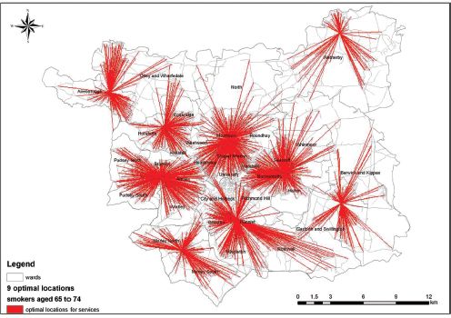
FIGURE 11.2 Nine optimal locations for stop-smoking services to target smokers aged 65–74 most effectively by using a location-allocation model
TABLE 11.1 Summarised information for nine optimal locations for stop-smoking services based on the location-allocation model to target estimated smokers aged 65–74

One of the UK government targets is also to reduce smoking rates in more disadvantaged areas. Heavy smokers (people who smoke 20 or more cigarettes a day) are mainly distributed in more disadvantaged areas where there are also high rates of morbidity and mortality from lung cancer. The third example of a model run uses the location-allocation model to find optimal locations for four additional stop-smoking services (where the number of services is chosen randomly for demonstration purposes) if additional money became available to target heavy smokers (Figure 11.3). To run the location-allocation model, the demand, supply and distance elements have to be set up as before. Demand here relates to a simulated population who smoke 20 or more cigarettes a day, and the centroids for the location of these smokers are calculated for all output areas in Leeds using ArcGIS. The supply items are the 19 stop-smoking services most often available on a typical day. These existing 19 clinics are set up in the way that the location-allocation model has to select these locations even if better locations could exist. All other locations are set up to be a possible location, which means that the model will find four optimal locations in addition to the 19 existing ones (by, as usual, minimising the distance travelled). The distance element remains a road network as it is more accurate than straight-line distance and the results are shown in terms of travel length. The blue dots on the map represent the existing 19 frequently open clinics and the red lines show the areas that the 23 stop-smoking services would now cover (19 existing plus four new ones). The four red spiders without blue dots are the best new locations. The model wants to locate these additional stop-smoking services in the north-west, west, north-east and east of Leeds. This shows the ‘untapped’ demand from heavy smoker residents in these areas. When adding four additional services, the average distance a smoker would need to travel is 2.2 km, whereas the furthest distance is 9.4 km.
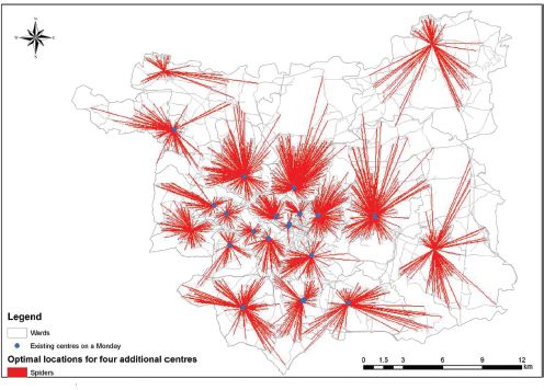
FIGURE 11.3 ‘Optimal’ locations for four additional stop-smoking services based on the number of simulated heavy smokers
A location-allocation model for police stations in Kuwait
Our second example concerns the location of police stations in Kuwait. This time the maximum coverage model will be used. In addition, the models are used to reduce the number of existing police stations, in order to save resources and concentrate services at fewer, larger centres. In many parts of the world, governments are attempting to save money by reducing expenditure on public services. In the UK, for example, the number of police stations was reduced by 630 between 2002 and 2012.
To set up a model for Kuwait the following datasets are required:
• location of police stations: this file also includes police station attributes (for 2011);
• districts file: this includes 83 census polygons, alongside the total population and crime rates within each district;
• roads network file: these roads are attributed as uni- and bidirectional.
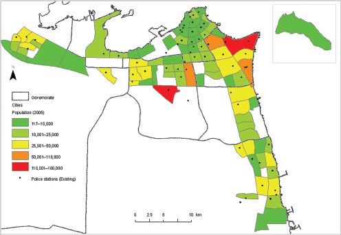
FIGURE 11.4 Distribution of existing police stations in Kuwait
Source: Kuwait Institute for Scientific Research 2011
Figure 11.4 shows the existing locations of police stations in Kuwait. As can be seen, all government municipalities or governorates in Kuwait are very well covered by existing police stations. However, the number varies from one governorate to another based on the size of population as well as the nature of each governorate (administratively and economically). For example, the Capital governorate (the capital of Kuwait located in the north-east of Figure 11.4), is the most important governorate in Kuwait in terms of administrative importance and hence has a high number of stations per head of population. There are 21 police stations located in this governorate, although the felony offence rate in 2005 was relatively low; there were 192 crimes in a population of 244,453 in 2011. In comparison, Mubarak Al-Khabeer (centre east in Figure 11.4), which is the newest governorate, has just two police stations. Similarly, Jleeb Al-Shiyoukharea has one police station to serve about 180,000 people. The crime rate here is particularly high because of the presence of many poor, marginal and manual labourers of non-Kuwaiti origin located together in a very overcrowded area. This area is coloured red in the centre of Figure 11.4.
Given limited resources, the location-allocation model can be used to reduce the number of police stations, as well as locating them more optimally in terms of the population and the number of crimes committed. The number of police stations needed is chosen as 15, despite the fact that the current number of the existing police stations is more than 50, as can be seen in Figure 11.4. Although this is an arbitrary number, it would reduce the provision by two-thirds and save considerable resources (whilst at the same time still providing a good geographical spread of stations across Kuwait). By applying the maximum demand model, most areas in the governorates of Kuwait could be covered by the new pattern of police stations (Figure 11.5). Between two and five minutes’ travel time is considered an appropriate response time for an emergency services facility, especially a police station (Tong and Murray, 2009). Therefore, the model worked on the constraint that approximately three minutes by car with a speed limit of 80 kilometres/hour is an ideal time response, with a maximum coverage of 4 km serving as a buffer. Figure 11.5indicates that, using three minutes by car, the majority of major districts can be covered by police stations.
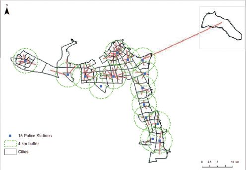
FIGURE 11.5 The proposed locations of police stations in the governorates of Kuwait, produced by Arcinfo Workstation
Conclusion
This chapter has described the use of location-allocation models for facility location. The models find the optimal location of X facilities (where X is determined by the planner) to minimise the distance travelled by users of those facilities. Models typically minimise total distance travelled by all users or ensure that no user is further from a predefined distance to their nearest facility. Given that competition between facilities is more difficult to incorporate into these models, they are typically used more prevalently in public service facility location than in commercial applications. The examples given in the chapter show how they can be used for important application areas such as health care and emergency planning. They are ideally suited to be an integral part of modern GIS, where the spatial data for the models can be pre-prepared and the results visualised in easy to interpret forms. There is no doubt that they are an important element within applied geocomputation and will continue to be refined in the future for even more sophisticated application areas.
FURTHER READING
It is always good to read original sources. One of the earliest and most cited references concerning location-allocation models is Cooper (1963, 1964):
• Cooper, L. (1963) Location-allocation problems. Operations Research, 11(3): 331–343.
• Cooper, L. (1964) Heuristic methods for location-allocation problems. SIAM Review, 6(1): 37–53.
A useful single collection of different applications of location-allocation models is Ghosh and Rushton (1987):
• Ghosh, A. and Rushton, G. (1987) Spatial Analysis and Location-Allocation Models. New York: Van Nostrand Reinhold.
A complementary article dealing with public sector applications, especially in relation to health planning, is Tanser et al. (2010):
• Tanser, F., Gething, P. and Atkinson, P. (2010) Location–allocation planning. In T. Brown, S. McLafferty and G. Moon (eds), A Companion to Health and Medical Geography (pp. 540–566). Oxford: Blackwell.
Richard Church and Alan Murray have made many innovative contributions to location-allocation modelling over the years. Church and Murray (2009) is a nice summary of these many advances, but also shows how the technique can be embedded more broadly in GIS and spatial analysis, especially for business site location:
• Church, R.L. and Murray, A.T. (2009) Business Site Selection, Location Analysis, and GIS. Hoboken, NJ: John Wiley.