Geocomputation: A Practical Primer (2015)

PART IV

EXPLAINING HOW THE WORLD WORKS

12

GEOGRAPHICALLY WEIGHTED GENERALISED LINEAR MODELLING

Tomoki Nakaya

Introduction

One of the most popular approaches to statistical model building is regression analysis. Here, we would associate a response variable we wish to predict with explanatory variables, using an assumed relationship such as a linear function. We fit the models to the observed data statistically, and then use the model to infer the properties of underlying processes hidden within the dataset. This chapter focuses on a specific type of regression modelling for spatial analyses, namely geographically weighted regression (GWR), and its extended form, semi-parametric geographically weighted generalised linear modelling (S-GWGLM). Such models replicate the geographically varying aspects of the association between the response and explanatory variables. The S-GWGLM modelling framework is implemented in GWR4, a free Microsoft Windows application, which we introduce in the case study part of this chapter.

GWR captures smoothed geographical variations in the relationships between variables using kernel-based non-parametric regression. This technique is based on the premise that ‘processes in different places are likely to be more similar as the places become closer together’. In particular, mapping the estimated coefficients of GWR models enables us to see the geographical structure of the spatial heterogeneity in the processes. In this sense, GWR is considered a tool of exploratory spatial data analysis (ESDA). ESDA lets us visually explore and infer the localised nature of geographical processes. Figure 12.1 shows a conceptual image of GWR.

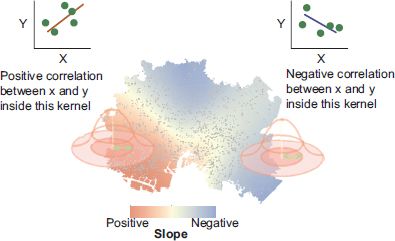
FIGURE 12.1 The concept of the GWR approach

Since the first seminal papers of GWR (Brunsdon et al., 1996; Fotheringham et al., 1996), many theoretical and applied studies of GWR have used the technique in fields such as geography, economics, ecology, epidemiology, and applied statistics; and Fotheringham et al. (2002) provides the most comprehensive guide to GWR. This chapter focuses on two important extensions of GWR (Nakaya et al., 2005, 2009):

1. Geographically weighted generalised linear modelling (GWGLM): GWR was proposed originally as an extension to the ordinary regression model to predict a continuous variable with a Gaussian (normal) error. However, when predicting a non-continuous variable, it is more appropriate to use different regression models, such as a logistic regression model for binary data, and a Poisson regression model for count data. Using a linear predictor, these regression models are integrated as generalised linear models (GLM: McCullagh and Nelder, 1989). Then, by integrating GLM and GWR, GWGLM models estimate binary and count data with coefficients that vary geographically.

2. Semi-parametric framework of GWR/GWGLM (S-GWR/S-GWGLM): A semi-parametric model is a regression model that combines non-parametric and parametric terms. In the case of GWR/GWGLM, a semi-parametric model mixes terms of geographically varying/local coefficients and fixed/global coefficients. This technique is more flexible than GWR/GWGLM. By fixing some effects as global rather than local, we can reduce the complexities of local relationships. This, in turn, may enhance the readability of geographically varying relationships, as well as the predictive performance of the model. Importantly, it also enables model comparisons, which we can use to determine which explanatory effects on the response variable are fixed globally and which vary geographically in GLM.

The following section explains S-GWGLM models in more detail; it then presents an implementation of the modelling framework using GWR4 by applying semiparametric geographically weighted logistic regression (S-GWLR) to a place-attachment dataset in a citywide geographical setting.

Outline of the method

Generalised linear models are a framework that covers a wide range of regression models that use a linear predictor and probability distributions from the exponential family. Suppose we have an ordinary regression model:

where y_i and x_ki are the response/dependent and kth explanatory/independent variable for sample/area i, respectively. β_k is the kth coefficient to be estimated; β₀ is the intercept, and we assume x_0,i = 1 for all i. In addition, ε_i is the error term that describes fluctuations not explained by the linear relationship of the explanatory variables. The error term is assumed to follow a normal distribution, with a mean of zero and variance of σ². The error distribution is represented by N(0, σ²).

In the GLM framework, a model has three components: the stochastic component of the prediction, the linear predictor using explanatory variables, and the link function that monotonically and continuously transforms the expectation of the response to the linear predictor. We can rewrite the ordinary regression model to represent these components as follows: the stochastic component is given by

for the systematic component, we have the linear predictor

and a link function

Equation (12.2) means that the prediction of the model follows a normal (Gaussian) distribution, with mean μ_i and variance σ². Equation (12.3) is the linear predictor that reflects the systematic component of the model prediction. Equation (12.4) tells us that the link function is the so-called ‘identity function’, which means that the expectation of the model’s prediction on the response is the same as that of the linear predictor.

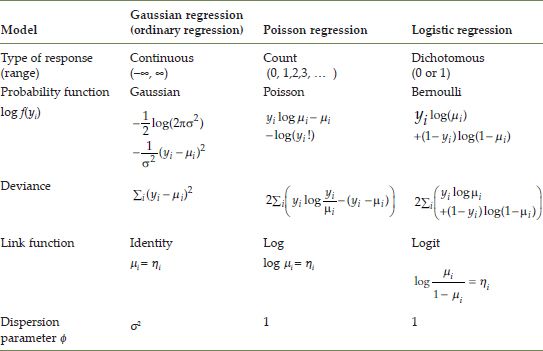
All GLM use linear predictors, but there are variations in the stochastic components and link functions. The most popular modes of GLM include Poisson regression for count data modelling and logistic regression for binary (dichotomous) data modelling. Table 12.1 summarises the three most popular GLM models.

With regard to the stochastic component, the model prediction is assumed to follow an exponential family distribution. The generic form of the distribution is as follows:

where f (y_i) is the probability distribution function that evaluates the likelihood of observation y_i, given its model-based estimate using the two parameters η_i and Φ. Therefore, we refer to the distribution function, f, and its log transformation, log f, as the likelihood and log-likelihood function, respectively. The function has three functional components, a, b and c, which are defined for each type of probability distribution.

TABLE 12.1 Three popular GLM models

Specification of GWGLM and S-GWGLM

GWGLM is a variant of GLM that includes coefficients that vary geographically. In this case, we replace equation (12.3), representing the linear predictor, with

In this model, the coefficients vary depending on the geographical coordinate of the sample geographical position i, (u_i, v_i). In the ordinary regression model, all coefficients model fixed/global effects, which remain spatially unchanged. However, these geographically varying coefficients model local effects.

There are three major modes of GWGLM that can be implemented in GWR4. Firstly, the Gaussian regression model is equivalent to conventional GWR. Here, equation (12.4) is replaced by

Secondly, the geographically weighted Poisson regression (GWPR) is μ_i = η_i(u_i, v_i)

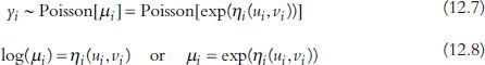
Poisson[μ_i] denotes the Poisson distribution with mean μ_i. In the Poisson regression model, a zero or positive integer represents a response count. It is worth noting that the log link transformation ensures that the expected value is non-negative. The Poisson regression model often includes one additional term, called the offset, ρ_i:

The response count is usually examined by the ratio of the count to the size of the collected samples. For example, suppose the count is the number of deaths in a population in an epidemiology study. In this case, the offset term, ρ_i, can represent the expected size of the outcome or the size of the population at risk at position i. Therefore, we can interpret exp(η_i) as the rate of the outcome occurrence. For more information, see the application of GWPR/S-GWPR to spatial epidemiology in Nakaya et al. (2005).

Thirdly, geographically weighted logistic regression (GWLR) is given by

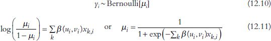
In this model, the response is either 0 or 1, so μ_i should be between 0 and 1. We obtain this condition using a logit function. Bernoulli[μ_i] denotes the Bernoulli distribution with parameter μ_i. This simply means that y_i is expected to be 1 with a probability of μ_i, and 0 with a probability of 1 – μ_i. For an application study, see Atkinson et al.’s (1993) application of GWGLM to geomorphology.

We refer to the semi-parametric variant of the models, S-GWGLM, as mixed GWGLM models, because both local and global effects are occur in one model:

where z_i,l is the lth explanatory variable for area i, and its coefficient, γ_l, is assumed to be fixed. GWGLM is equivalent to the so-called partially linear models in local regression. One reason for using this kind of model is that we occasionally want to analyse varying effects by adjusting other effects. If we set all explanatory effects as global terms, except for the intercept term, we can consider the geographical distribution of local intercept estimates as spatially smoothed areal effects, adjusted by the other explanatory variables. It is also useful to judge if a term should be a local or global term, as we will discuss later.

Estimating coefficients of GWGLM and S-GWGLM

GWR estimates the local coefficients by repeatedly fitting the regression model to a geographical subset of the data using a geographical kernel weighting. Imagine a circle of a certain radius measured from the regression point at which the coefficients are to be estimated. Fitting the original regression model to the subset of the data within the circle provides estimates of the local coefficients. By repeating the local fitting of the regression model for the regression points, we obtain the set of local coefficients for the points. Instead of using a simple circular window, GWR uses a geographical kernel weighting, which yields a fuzzy local subset to generate a smoother surface for the local coefficients. In essence, the kernel weighting is used to evaluate the goodness of fit of the predicted response to the observed response, giving more importance to locations that are nearer to the regression point (cf. Figure 12.1).

GWGLM uses geographically weighted maximum likelihood estimation (GWMLE) to estimate the local coefficients of the ith regression point. To do so, it solves the following maximisation problem of the geographically weighted log-likelihood model:

where the symbol ^ refers to the estimate, is the set of estimated coefficients focusing on regression point i, and d_ij is the distance between locations i and j. The dispersion parameter of distribution Φ is σ² in the case of the Gaussian model, while the Poisson and logistic regression models usually assume Φ = 1 a priori. The numerical process used to estimate the local coefficients is the geographically weighted variant of the scoring algorithm (Fotheringham et al., 2002).

The geographical weight of the jth observation at the ith regression point, w_ij, is introduced here as a non-negative and monotonically decreasing function of the distance between ith and the jth location. A popular choice is the fixed Gaussian kernel function

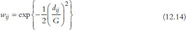
where G is the bandwidth parameter that controls the local geographical extent of the weighting. Here, the fixed kernel means that a fixed G is applied for all local model fitting.

A popular alternative is the following adaptive bi-square function:

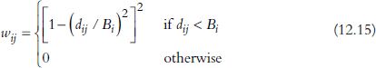
Given that M is the bandwidth parameter applied for all local model fitting, the bandwidth, B_i, which is dependent on regression point i, is defined as the distance to the Mth nearest observation point from the regression point. Adaptive kernels are useful in preventing unreliable coefficient estimates because of the number of observations in local subsets. This is particularly true when the distribution of the regression points is highly uneven. We can also use adaptive Gaussian or fixed bi-square functions.

Estimation using S-GWGLM is more complicated than GWGLM. In essence, the method employs a ‘back-fitting procedure’ (Hastie and Tibshirani, 1990), which repeats the following steps until the estimation converges: (i) estimate the local coefficients given the global coefficients, based on GWMLE; and (ii) estimate the global coefficients given the local coefficients, based on the usual maximum likelihood estimation (Nakaya et al., 2005). It is also possible to derive indicators for model diagnostics, including standard errors for the coefficients and the degrees of freedom of the model based on the estimation principle.

The deviance is an indicator of the goodness of fit of the fitted model, based on the log-likelihood in GLM. The (residual) deviance of a fitted model, D_fitted, is defined as

This is the difference in the log-likelihood between the fitted model and the full/saturated model. The full model has a parameter for each observation, so it fits the data perfectly, but has no degrees of freedom. Here, a better fit between model and data means a smaller deviance. A related statistic, with a limited range from 0 to 1, is the pseudo R-squared or ‘percentage of deviance explained’:

Here, D_null is the deviance of the null model, which only has a constant term, and no explanatory variables. In the case of the Gaussian model, this is equivalent to R-squared. If the model better fits the data, the value of PD increases.

Bandwidth selection

The bandwidth size regulates the GWGLM model complexity because the bandwidth controls the degree of variability of the estimated coefficients. An extremely small bandwidth means we repeat the local model fitting to a very small geographical subset of the data. In this case, the estimates of the coefficients are likely to fit the data well, but might be unreliable because the estimates will show large variances due to the lack of degrees of freedom (DOF) in the local model fitting. On the other hand, using a large bandwidth may ignore meaningful spatial variations in the coefficients when the true distribution varies spatially. In this case, a model using an excessively large bandwidth yields strongly biased estimates. Therefore, selecting a bandwidth involves a trade-off between the goodness of fit and DOF, or between the bias and variance of the model estimates.

One solution is to find the optimal bandwidth size using a model selection criterion, such as cross-validation (CV), Akaike’s information criterion (AIC), or AIC corrected for a small sample size (AICc). This concept is shown in Figure 12.2. In particular, AICc is useful when modelling relatively small DOF, as often encountered in non-parametric regression, even for non-Gaussian models (Burnham and Anderson, 2002). AICc is defined as follows:

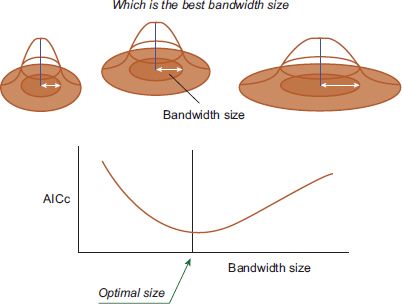
FIGURE 12.2 How to decide on the optimal bandwidth size

where denotes the log-likelihood of the fitted model, representing its goodness of fit. The better the model fits the observed data, the smaller the log-likelihood. Here, q represents the number of parameters in the model. Given p as the total number of coefficients in the linear predictor, q = p for Poisson and logistic regression models, and q = p + 1 for Gaussian models. This is because the dispersion parameter, σ², is estimated as . A smaller value of q means that the model is simpler, and hence has smaller DOF. The smaller the AICc of the model, the better the predictive performance of the model will be.

However, it is not straightforward to apply the criteria to GWGLM, because the geographic variability of coefficients is not specified as an explicit function with independent parameters. Therefore, effectively equivalent numbers of parameters are derived from local regression theories (Loader, 1999), and use the values for model selection (for details, see Nakaya et al., 2005).

Geographical variability test of coefficients

An advantage of S-GWGLM is that we can incorporate a fixed/global effect of a subset of the explanatory variables on the response variable based on prior knowledge. However, it is not always obvious which coefficients should be assumed as fixed or variable. A natural way to overcome this difficulty is to conduct empirical model comparisons of different S-GWGLM models using different combinations of fixed and varying coefficients.

To assess the variability of the kth coefficient in a GWGLM model, we compare two models; the fitted GWGLM model (pivot model) and the model in which only the kth coefficient is constant, while the other coefficients vary spatially (k-fixed model). If the pivot model is better than the k-fixed model according to a model comparison criterion such as AICc, we consider the variability of the kth coefficient to be statistically supported. If we have the AICc of the pivot model, AICc_{pivot: k-varying}, and the k-fixed model, AICc_k-fixed, we can calculate the difference between the two as

If this quantity is positive, the k-fixed model is better than the pivot model. In this case, it is better to use the kth term as a global term rather than a local term. When the absolute size of AICc difference is within 1 or 2, there is essentially no difference between the two. A rough rule of thumb is that, when the absolute difference is larger than 4, the judgement is more clearly supported (Burnham and Anderson, 2002).

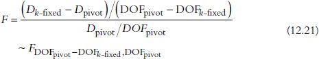
When comparing the nested models, hypothetical testing is also possible. When the dispersion parameter for the GWPR and GWLR is set to 1, the difference in deviance between the two models follows an approximately chi-square distribution under the null hypothesis that there is no difference in the performance of the two models. The DOF of the chi-square distribution is the difference between the DOF of the two models:

GWR4 computes the equivalent statistics for (S-)GWGLM. In the case of the Gaussian model, it is better to evaluate the stochastic error for the inference of the dispersion parameter. In this case, the F-statistics approximately follow an F distribution under the null hypothesis that there is no difference in the performance of the two models (Mei et al, 2006):

In both hypothesis tests, when the null hypothesis is rejected, we can say that the term shows significantly geographical variation at the significance level used for the test.

Automated model building

GWR4 contains two separate fitting techniques for automated variable selection in the S-GWGLM models. One is the LtoG (from local to global term) variable selection routine, which executes a series of model comparisons to search for the optimal combination of varying and fixed terms, given the explanatory and response variables. The concept is similar to that of stepwise variable selection:

Step 1: Begin with an (S-)GWGLM model with local terms and varying coefficients as a pivot model.

Step 2: Try to fit a series of model by switching the varying local terms to global, one by one, and establish which switch gives the best performance in terms of the model selection criterion.

Step 3: If the best term from step 2 improves the model performance, the pivot model is updated by changing the relevant local term to a global term.

Step 4: Repeat steps 2 and 3 until no further improvement is possible by switching any terms from being local to global.

An alternative model selection procedure, also implemented in GWR4, is GtoL (from global to local term). This is the reverse procedure to that described above. In this case, the default model is the global model (or an S-GWGLM model), and the first round of model comparisons allows each parameter in turn to be spatially varying. Here, model selection occurs in the same way. In other words, we select an optimal model based on the model selection criteria, and then repeat this until no further improvement is possible.

A practical S-GWGLM analysis of place attachment using GWR4

To demonstrate the S-GWGLM framework, this section uses a case study to analyse place attachment using S-GWGLM modelling. Place attachment refers to the affective bonds that link people to a certain place (Lewicka, 2011). The concept is closely related to ‘topophilia’ and ‘sense of place’ in human geography (Tuan, 1974), and is associated with people’s self-identity, well-being, and social participation. The data are taken from an internet-based questionnaire survey conducted in 2009 by a social survey company. The respondents relate to residents of the central Tokyo metropolitan area, consisting of 23 wards of Tokyo and the surrounding cities (n = 1393).

Although place attachment is a multi-dimensional construct, the indicator we use here is based on a simple question in the survey: ‘Do you feel attached to the neighbourhood in which you live?’ Respondents could indicate one of five choices {1, yes; 2, yes, weakly; 3, hard to say; 4, no, weakly; 5, no}. In this analysis, we focus on the following recoded dichotomous variable representing the response: PA (place attachment) = {0 if choice 3, 4, or 5 is selected; 1 if either 1 or 2 is selected}. Therefore, the research question examines the association between the place-attachment response and the other explanatory factors, and how this association varies geographically.

There are three explanatory variables in this case study. LIVLEN represents the length of time the respondent has lived in their current residence, and is defined as {0, less than 10 years; 1, greater than or equal to 10, but less than 20 years; 2, greater than or equal to 20 years}. The longer a person has lived in a place, the more likely it is that place attachment will occur. OWNH indicates if the respondent owns his or her house {0, no; 1, yes}. House ownership may enhance place attachment because a person who owns a house expects to be there for a long time. Therefore, we expect OWNH to be positively associated with place attachment. Finally, UPRE indicates whether the respondent prefers living in the suburbs or city centre {0, prefers living in suburbs or hard to say; 1, prefers living in city centre}. UPRE is based on the question ‘If you could choose between living near the city centre and in the suburbs of the city, which would you prefer?’ Since the study area is the core region of the metropolitan area, the preference for a lifestyle that depends on an urbanised environment is thought to be positively correlated to the place-attachment indicator. The result of the global logistic regression model generally supports these expected effects, though the effect of LIVLEN is insignificant. This may be because LIVLEN is correlated with OWNH.

The numbers in parentheses below the coefficients are the standard errors of the estimates. Note that the data file must contain the geographical coordinates. Although the coordinates in the sample data set are not precise residential locations, being randomly perturbed with spatial constraints (the maximal size of the dislocation is about 5.5 km), the results are essentially the same as when we use the original coordinates.

Considering S-GWLR models

The simplest GWLR model is a constant model without any explanatory variables. In this case, the estimator takes the following simple form:

In the case study, this is a local ratio of ‘the number of people feeling place attachment’ to ‘the number of people feeling weak or no place attachment’ around the point (u_i, v_i). The general distributional pattern of the local ratio using this estimator is a good way to start exploring possible geographical effects on weak place attachment among residents. However, some analysts may consider adjusting LIVLEN to see this geographical variation in case the effect of the length of residence is established. In this case, we use the following S-GWLR (Model 1):

where the effect of length of residence is set as a global term so that the geographically varying intercept term, , is considered as the ratio described earlier, but adjusted by the sample’s length of residence. We can also view the model as a special logistic regression model by considering spatially autocorrelated unknown factors, which are captured by the varying intercept term.

To further explore any geographic variability in the explanatory variables, we can compare the above models with the following GWLR (Model 2):

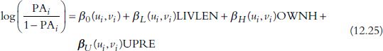
The final model used here (Model 3) is obtained from the LtoG automated model building process, based on Model 2:

where the effects of LIVLEN and OWNH are considered to be global. To interpret the coefficient of logistic regression, it is common to use the exponential form of the coefficient (e.g. , which represents the odds ratio (OR) of the response, shown as PA_i/(1–PA_i) for an increase of +1 in the explanatory variable, x_k.

Using GWR4

GWR4 was developed to implement S-GWGLM modelling with a GUI-based interface. It uses tabbed sub-windows so that a modelling session proceeds intuitively in a step-by-step manner. The program also offers a wider range of options related to GWGLM, including geographical variability assessment and the automated variable selection routines explained earlier. The program operates within a Microsoft Windows environment and is based on the .Net Framework 4.0.

GWR4 consists of five steps when running a model: Data, Model, Kernel, Output, and Execute. Each step has a corresponding tab (see Figure 12.3). The user first opens the data file in the Data tab, and then moves to the Model tab to specify the model. Figure 12.4 demonstrates the various settings available in the Model tab for Model 4. The dataset opens in the File tab, and the list of fields/variables appears in the centre box. If you wish, you can move fields to other boxes to specify the response/dependent variable, the explanatory variables as geographically varying (local term) or fixed (global term), and at least two geographical coordinates. In the case of GWGLM, the model type should be changed from Gaussian to logistic. Geographical variability testing and automated model building are both optional. Since an S-GWGLM model requires a much longer computational time than the corresponding GWGLM model, these options may take a relatively long time to complete, particularly when implemented as part of automated model building.

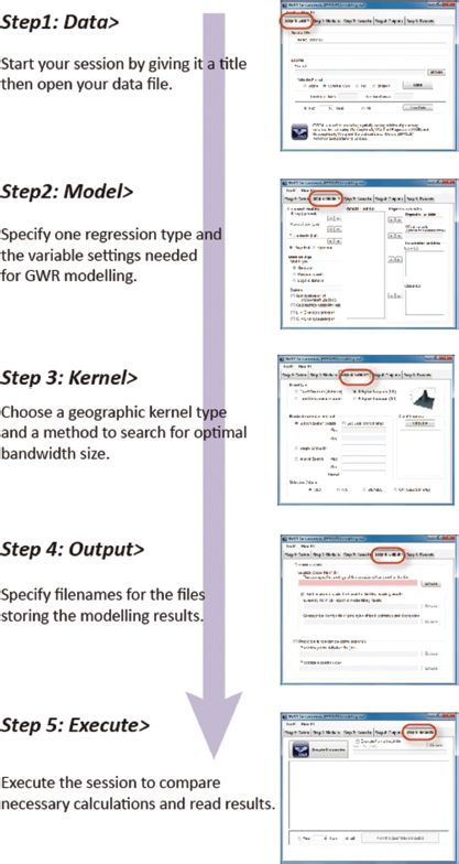
FIGURE 12.3 The steps in a GWR modelling session

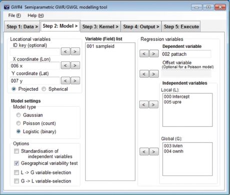
FIGURE 12.4 Screenshot of the specification in the Model tab

In the Kernel tab, the default setting is to use an adaptive bi-square kernel and to find the optimal bandwidth using the ‘golden section search’ option, based on AICc. However, these settings can be changed. Although the golden section search is a useful way to automatically find the optimal bandwidth, it is not always straightforward to find adequate initial bandwidths. Since binary data is less informative than continuous and count data, model fitting using a small bandwidth often fails to converge. In a small subset of data, the variation in the response and explanatory variables is likely to be too small for model fitting. GWR4 automatically adjusts the search range using trial and error. This might be time-consuming in the case of GWLR. Therefore, we recommend that a user specifies the minimum bandwidth for the search after several trials. In the sample data analysis, the nearest 400 samples for an adaptive bi-square kernel are used as the minimum search range for the bandwidth, as shown in Figure 12.5. Note that, when the optimal bandwidth in the routine is the minimum bandwidth size, the software generates a warning message in the summary output files.

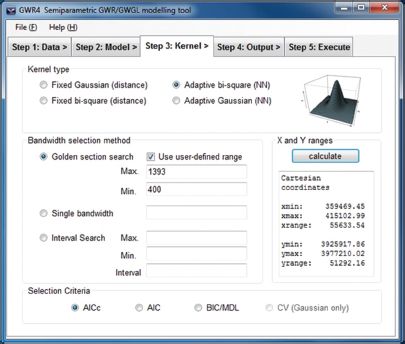
FIGURE 12.5 Screenshot of the specification in the Kernel tab

In the Output tab, the user specifies a file name for the session control file. This file saves the settings entered in the previous tabs, including the data and geographic kernel information. The file can be reused later by opening it from the File menu or running the model from the command line. Finally, to run the model, click the ‘Execute’ button in the Execute tab. The output is displayed on the screen, and is stored in the files specified in the Output tab.

As noted earlier, there are two output files that contain the modelling results. The summary file contains the general summary information of the fitted model, and comprises:

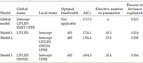
The supplementary material provides a sample of the summary file. The indicators used to evaluate the statistical performance of the fitted model are available in part (iv) of the summary file. Table 12.2 summarises the indicators for the fitted models in the case study.

TABLE 12.2 Summary of fitted geographically weighted logistic regression models

If the user selected a variability test and automated model building, these results are added to the bottom of the summary. For example, Table 12.3 shows the reported result of the geographically varying test when applying Model 3. In this case, the coefficients all vary geographically. The difference in the AICc, shown as ‘Difference of model selection criterion (AICc)’ in Table 12.3, suggests that the coefficients of LIVLEN and OWNH are better as fixed, while the intercept and the coefficient of UPREF are better as geographically varying. Rounding up the fractions in the difference in the DOF, we can use the chi-square distribution with DOF = 7 for the hypothetical test. The rejection region of the chi-square test with DOF = 7 and a significance level of 0.05 is ∆D(k)>14.07, according to chi-square distribution tables. Based on ∆D(k), shown as ‘Diff of deviance, ∆D(k)’ in the table, we can conclude that the geographic variability of the intercept and the coefficient of UPREF are statistically significant at the 5% level.

The geographic listwise output file stores the estimated coefficients, their standard errors, and local model diagnostic indicators, including the local version of percentage deviance explained. Figure 12.6 shows the length-of-residence adjusted ratio for the place attachment rate as the distribution of , using Model 1. The figure shows a general trend that the values are high in the central and western part of the region. In other words, people living in these regions are more likely to have strong place attachment than those in other regions. The distribution of the z-value (pseudo t-value), defined as the local coefficient divided by its standard error, is shown using contour lines on the map. Broadly speaking, the values are mostly above 1.98 or below –1.98, which suggests that is not equal to zero at the 5% level.

TABLE 12.3 Statistics for the geographical variability tests for local terms of the geographically weighted logistic regression model (Model 2)

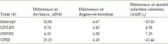
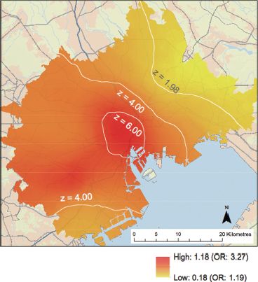
FIGURE 12.6 Distribution of the intercept parameter of Model 1 (OR: local odds ratio of people feeling place attachment adjusted by the length-of-residence effect)

Model 3 attains the lowest AICc and is considered the best model in this analysis. Using this result, Figure 12.7 shows the distribution of and the effects of UPREF, which exhibits significant geographical variability. The value in the central part of the study area is clearly positive, indicating that people who prefer living in a city centre are likely to exhibit place attachment. On the other hand, the peripheral parts of the study region show negative values. This may reflect that people living in peripheral regions perceive the neighbourhood environment as being less urbanised, and those who aspire to a city-centre lifestyle are therefore likely to be less satisfied. This case study shows that the development of an affective feeling of bonding with a living area is inhibited if there is a disagreement between the expected and experienced neighbourhood environment. In addition, the case study also shows the utility of the S-GWLR, which enables us to infer the geographic context associated with such a psychological disagreement about a living place.

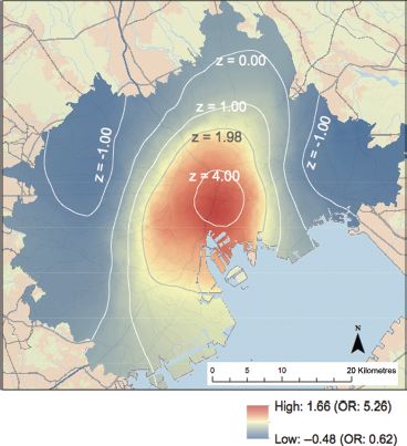
FIGURE 12.7 Distribution of local effects of UPRE on weak place attachment according to Model 3

Conclusion

This chapter has introduced the GLM-based semi-parametric geographically weighted regression (S-GWGLM) modelling framework. This framework allows us to mix geographically varying and fixed coefficients in a generalised linear model. It also allows us to explore which explanatory terms should be varying or fixed by comparing possible S-GWGLM models. GWR4 is a computer application that was developed as a platform to implement S-GWGLM modelling. The software includes the new methods of assessing geographical variability for estimated coefficients and automated model selection, enabling the user to search for an optimal combination of fixed and varying explanatory terms in a model. While GWR4 currently only fully supports S-GWGLM functions, other recent software applications are equipped with other types of advanced GWR functions. For example, ArcGIS provides a function to integrate GWR model fitting into its cartographic display, and the R packages spgwr and GWmodel provide a wide array of GWR variants and related tools to manage several problems in local modelling, such as local collinearity or outlier problems. Note that geographically local properties explored using these tools are closely related to the mode of spatial thinking that emphasises geographical context (Fotheringham, 1997). Therefore, meaningful interpretations of the results from these tools may challenge the user’s spatial thinking ability, based on their geographical knowledge and technical understanding.

FURTHER READING

Fotheringham et al. (2002) provides a most comprehensive guide of GWR and its extensions:

Fotheringham, A.S., Brunsdon, C. and Charlton, M. (2002) Geographically Weighted Regression. Chichester: Wiley.

GWR can be considered as a type of ‘local spatial analysis’ which has been proposed to extract geographically local properties in geospatial information. Lloyd (2011) is a useful overview on a wide array of modern local spatial analyses including GWR:

Lloyd, C.D. (2011) Local Models for Spatial Analysis, 2nd edn. Boca Raton, FL: CRC Press.

Web resources

Information about GWR, including the GWR4 download sites, is available at the following GWR portal sites: https://geodatacenter.asu.edu/gwr_software (GeoDa Center for Geospatial Analysis and Computation, Arizona State University) and http://ncg.nuim.ie/ncg/GWR (National Centre for Geocomputation, National University of Ireland, Maynooth).

ACKNOWLEDGEMENTS

This work was supported by JSPS KAKENHI Grants 20298722 and 24300323. The author wishes to thank Stewart Fotheringham (Arizona State University), Martin Charlton (National University of Ireland), Chris Brunsdon (National University of Ireland), Paul Lewis (National University of Ireland), and Jing Yao (University of St Andrews) for their kind support and collaboration on the development of GWR4.