Geocomputation: A Practical Primer (2015)

PART IV

EXPLAINING HOW THE WORLD WORKS

13

SPATIAL INTERACTION MODELS

Karyn Morrissey

Introduction

Both conceptual and analytical methods for evaluating spatial flows have traditionally been based on how distance and transportation options impede an individual’s travel decision-making. This chapter outlines the method of spatial interaction modelling, which allows a full set of complexities involved in travel decisions to be encompassed within a single framework. Such complexities might include the demographic and socio-economic profile of the populations under study, the profile or ‘attractiveness’ of the end destination, and travel cost – in terms of distance travelled and any impedances of the transport network. This chapter introduces those steps and data required to model flows of individuals from one destination to the next using spatial interaction models. A worked example in the spreadsheet package Excel illustrates a spatial interaction model estimating trips to hypothetical medical services in Liverpool.

An important requirement of product and service success, in both the private and public sector, is an understanding of how, where and when consumers access goods and services. Thus, the spatial flows of individuals to and from particular locations are important for planning likely users of new facilities or the demand for a certain product such as a new community health centre or a new retail park. Initial studies on spatial flows (or, more broadly, accessibility) attempted to assess flows in terms of transport opportunities alone (Jones, 1981). However, how an individual chooses to move across space is a much broader concept than transport availability alone. The work of Moseley (1979) moved away from the idea of mobility as a proxy for spatial flows and defined trip choices in terms of accessibility. Moseley (1979) asserted that accessibility is more than just the transport modes or distance involved in reaching a particular service; accessibility is also about the attributes of the people wishing to access a service, the attributes of the destinations and the means by which these opportunities are reached. Thus, to fully understand spatial flows, one must identify three components: the people wishing to travel, the potential places/opportunities to be visited and the distance/separation of people from these places/opportunities.

Further work by Joseph and Phillips (1984) classified access according to two categories, potential and revealed access. Potential access refers to a person’s ease of accessing these services based on existing conditions but does not warrant the utilisation of the service. Revealed accessibility, based on potential access, focuses on the actual use of services (Joseph and Phillips, 1984). Both types of access can be further classified into spatial and non-spatial access (Luo and Wang, 2003; Wan et al., 2012; Bissonnette et al., 2012) based on how the accessibility is influenced by spatial factors (e.g. spatial location and travel distance) and non-spatial factors (e.g. socio-economic status, or cultural background). Thus, to model spatial flows that represent a realistic pattern of human behaviour, how individuals chose to access services, both spatial and non-spatial considerations must be taken into account. Spatial interaction models (SIMs) involve determining through demand, supply and interaction information the attributes that promote flows of people and goods between different locations.

Modelling framework

Spatial interaction models have a long tradition of being used to estimate flows of people to service outlets (Birkin and Clarke, 1991; O’Kelly, 1986; Yano et al., 2000). For different consumers and destination choices, one can model the trade-off between spatial convenience (visiting an outlet close by) and the attractiveness of particular outlets (measured by proxies such as size, brand and quality of the service). Although there is a classical family of SIMs (Wilson, 1974), one model, the production-constrained SIM, has dominated the literature (Fotheringham et al., 2001; Clarke et al., 2002). Such models allow the user to estimate the trip end totals (revenue in shopping models, number of patients attending hospital or surgery in health-care models) and may be used by planners to locate or reconfigure new services. Thus, a production-constrained SIM may be used as a location model (Clarke and Wilson, 1994) From the outputs of these models, it is also possible to build a suite of accessibility indicators that measure how well served residents are for services under consideration (Clarke and Wilson, 1994; Clarke et al., 2002; Morrissey et al., 2008). Thus, such models can be used to quantify accessibility according to where individuals consume services as predicted by the SIM, and as such, provide a more realistic representation of access to services than, for example, simply taking the number of service outlets in a zone or estimating accessibility through a simple straight-line nearest facility type indicator.

The steps required to model an SIM and develop a suite of accessibility indicators may be broken down into six major processes:

• problem definition;

• model specification and data collection;

• travel impedance measurement;

• calculation of accessibility measures;

• interpretation and evaluation of the results;

• visualisation of accessibility values.

The first step is to define those spatial flows that are to be estimated. For example, do they relate to the number of potential trips to a new supermarket, or the demand for hospital services in a region? Within the model specification stage, this involves identifying what data you are going to use, both spatial and non-spatial. Spatial interaction analysis is typically a data-intensive process, and four pieces of information need to be included:

• definition of the spatial unit for analysis;

• definition of the socio-economic groups involved;

• the attributes of the destination;

• available modes of transport.

Sources usually include secondary data such as the census of population (as used in the example presented later in the chapter) and/or survey data. However, a key requirement of any dataset used for SIMs is that the data contain spatial referencing, such as an individual’s address or attached nested zone (census tract, etc.). Examples of SIMs relate to a range of spatial scales from the local (e.g. facilities in the neighbourhood), to regional (e.g. cities and their hinterlands) and inter-regional levels (e.g. connectedness of a region or country).

In practice the selected scale needs to be linked to the planning and policy decisions required at each level: within communities, neighbourhoods and larger administrative areas. For example, an aim of using SIMs to improve accessibility plans at the regional level does not always lead to improved accessibility at the local level. This means that a policy that is to be implemented at the regional level needs to have its ramifications examined at the local level to ensure that it does not hinder local level accessibility.

With regard to aspatial factors, it is not possible to identify every need for every group since there are potentially hundreds of combinations of socio-economic groups. However, to maximise the usefulness of spatial interaction modelling in policy and planning, it is important to categorise people and places as thoroughly as possible. Spatially referenced demographic and socio-economic data are typically available through the census of population for a country, or modelled surrogates such as those derived from large-scale rolling surveys (e.g. the American Community Survey). The types of opportunities offered at the destination sites are assessed through a variety of mechanisms depending on application area and include the prevalently used square footage of a retail park or the availability of certain opportunities at the destination (e.g. a course of higher education, or type of retail). The goal of any transport system is not mobility per se, but access to facilities. Private transport by car will invariably offer the best means of accessibility in many areas. However, there are a multitude of transport methods, from private car to public transport, walking and cycling. These options should be considered in a well-executed spatial interaction analysis.

The worked example illustrated in this chapter involves creating an SIM to estimate flows of individuals to five hypothetical medical practices across 12 output areas (OAs) in Liverpool. An OA corresponds to around 15 households. Thus, data at the OA level are required, and the best source of information about the characteristics of these zones is found within the Census of Population. Data on the number of doctors in each medical practice may be taken from the medical practices’ websites (attractiveness of the destination) or health-service databases. Travel impedance for the purpose of this worked example used Euclidean distance to calculate distance between the centroid of each OA and each of the medical practices, although road network distances could also be used, as these take travel conditions into account.

Travel impedance

Travel impedance represents the spatial separation between an origin, i, and a destination, j. Travel impedance can be measured in terms of travel distance, time or cost estimated by straight-line distance or network distance (Liu and Zhu, 2004). Due to the complexity of travel behaviour and data limitations, it is not always practical to have accessibility measures with a full range of travel options. Indeed, due to the complexities of measuring public transport, it is often assumed that an individual is travelling by private car (Liu and Zhu, 2004).

Factors that lead to travel impedance can be categorised under five headings: spatial, physical, temporal, financial and information. Spatial barriers relate to the distances involved in accessing required goods and services (Kwan and Weber, 2003). Time is an integral element of individual accessibility. This refers not only to the amount of time available to an individual for carrying out travel and activities, but also to the scheduling of activities throughout the day (Kwan and Weber, 2003). Thus, temporal barriers to accessibility arise within two contexts: firstly, when there is a mismatch between service times; and secondly, when the required travel times exceed some maximum threshold of practicability and acceptability. Temporal accessibility can be greatly improved by scheduling service delivery and transport provision jointly. In debates about the financial cost of travel as a factor affecting accessibility, the emphasis is often on affordability. As demand for public transport declines in rural areas, user costs increase, leading to increases in fares. Travel costs are a more significant barrier to access for some groups than others. Access to low-wage employment will only be practical if fares are low enough to make employment viable. As a result, people on low incomes tend to work closer to home. As incomes are lower in rural areas in general, this can lead to issues such as rural deprivation and social exclusion. Physical accessibility barriers are often perceived as being the easiest to understand, and they are classified in terms of the assistance that an individual needs to make a journey.

Calculating spatial flows using spatial interaction models

SIMs involve determining through demand, supply and interaction information those attributes that promote flows of people and goods between different locations. For different consumers, one can model the trade-off between spatial convenience (visiting an outlet close by) and the attractiveness of particular outlets (measured by proxies such as size, brand and quality of the service). SIMs differ in form from other model-based approaches to accessibility analysis in that they may be derived via entropy-maximising techniques (Wilson, 1974) or contingency table theory (Willekens, 1983), rather than Newton’s law of gravitational attraction. Entropy-maximising models are commonly used to find the most probable numbers of pairings x_ij between locations i and j given the number of origins, O_i, in location i and the number of destinations, D_j, in location j. Thus, the most probable macro-distribution is one that replicates the maximum number of micro-level events (Roy and Thill, 2004). Contingency table theory focuses on the pattern of association among variables and cross-classifies these interactions in a table of spatial interaction flows. Contingency tables are generally calculated via multivariate analysis such as log-linear models or logistic regression models.

There are four types of SIM commonly in use:

• Destination-constrained SIMs assume that the attributes of the supply point are known, that is, the locations of various service providers (supply points).

• Origin-constrained SIMs assume that the attributes of the demand point are known, that is, the location of households (demand points).

• Doubly constrained models assumes that the both the supply and demand point attributes are known.

• Unconstrained models assume that neither demand nor supply attributes are known.

Among these, the origin-constrained SIM is by far the most popular (Clarke et al., 2002; Morrissey et al., 2008). Models of this type allow the user to estimate the trip end totals (revenue in shopping models, the number of patients attending hospital in health-care models) and thus serve as location models. From the outputs of these models it is possible to build a suite of performance indicators to measure how well served residents are for the service under consideration (Clarke and Wilson, 1994; Clarke et al., 2002). Thus, these models quantify accessibility according to where they predict individuals consume services, and, as such, provide a more realistic representation of access to services than, for example, simply taking the number of service outlets in a zone or estimating accessibility through a simple straight-line nearest facility type indicator.

An example of an origin-constrained spatial interaction model is the following, which includes a worked example in Excel to estimate trips to a medical practice:

where T_ij is the flow of individuals from residential zone i to each service centre j, O_i is the demand for the service in a predefined spatial area i, such as a postcode or a ward, W_j is the attractiveness of outlet j, d_ij is the distance from the origin i to the destination j, β is a distance decay parameter and A_i is a balancing factor that ensures that

A_i is calculated as

The demand side (zone i) is usually represented as households or individuals aggregated into the smallest geographical output level available within the dataset. The supply element of the SIM represents the attractiveness of any given destination.

In this chapter the SIM described above is used to measure access scores from each of the OAs to their nearest medical centre using hypothetical data for Liverpool and a model developed in Excel. For the purpose of this chapter the attractiveness parameter for each health-care centre, W_j, is the number of practitioners in each health centre (a measure of how easy it is to be examined quickly). The demand variable, O_i, is the potential demand for medical services given the number of individuals with long-term illness in a particular OA. The distance variable, d_ij, is the distance from each OA centroid, i, to each medical practice, j. In the worked example in Excel, distance is calculated using the formula for Euclidean distance. However, it is important to note that the most accurate method of calculating D_ij is too use a network analysis tool in GIS. This allows road distance and increasingly temporal aspects to commuting such as congestion to be estimated for each origin–destination pairing. Figures 13.1–13.3 represent a worked example using our medical example within an SIM created using Excel. The spreadsheets used in this example are available as an online resource as part of this book. An additional spreadsheet presenting the formulas for each for each of the cells is also available, to aid students to develop their own SIMs.

It is possible to derive accessibility indicators from the predicted levels of interaction as calculated by an SIM. Such indicators can quantify accessibility according to where individuals travel to (as predicted by the SIM) and, as such, provide a more realistic representation of access based on the movements of individuals rather than simply on the geographical distribution of service outlets within a zone. In this section, two model-based performance indicators are described, and were first introduced by Clarke and Wilson (1994). The first type of performance indicator relates to individuals and households. These indicators are based on residential location and relate to the ways in which the individual is served by facilities. As such, these indicators can be used to estimate the effectiveness of service provision to individuals. The second type of performance indicator relates to service providers and the specific services that they provide. Thus, these indicators measure the efficiency of provision by service providers.

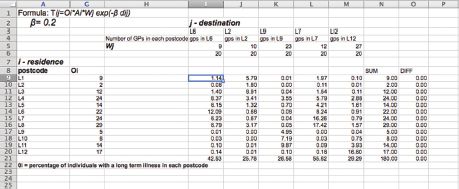
FIGURE 13.1 SIM output calculation in Excel

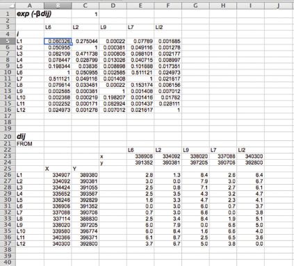
FIGURE 13.2 Calculation of distance using Euclidean distance (d_ij) and the distance decay parameter exp(–βd_ij) for the SIM

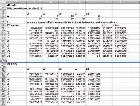
FIGURE 13.3 Calculation of SIM attractiveness parameter (A_i)

By identifying spatial variations in effectiveness and efficiency of provision, such performance indicators allow the targeting of resources to increase the efficiency of a service facility or to increase the effectiveness of service provision to households. To analyse accessibility of rural services, one needs to use both the efficiency and effectiveness indicators together. Using both indicators to analyse spatial interaction provides an understanding of how households and facilities are interdependent. Thus, these indicators allow planners to examine whether the problem is in the effectiveness of delivery to residential locations or in the efficiency of provision at facility locations.

The following model-based indicators measure the effectiveness of service delivery to residential areas. As such, they measure the aggregate level of provision and the level of provision per household, respectively. These indicators are important because the effectiveness of a provider in delivering its services is based on its size and location. The aggregate level of provision for a particular origin zone i is given as

This equation for estimating the aggregate level of provision for an area is calculated by dividing each SIM output (equation (13.1)) by the sum of all outputs for each zone j, where * indicates summation across all zones i. This is then multiplied by the attractiveness of zone j. The sum of all these values for residence zone i provides the aggregate provision for each zone i. This indicator ensures that even if an area does not have a service facility, the area will not have a zero accessibility score (unlike traditional indicators). In order to identify areas with low service provision it is necessary to relate this level of provision to the number of households in each area. For example, if service provision for a particular area is low, but population is also low, then the area may not be classified as a problem zone. On the other hand, if an area has relatively low provision and population is high, then the results of the model will identify it as a problem area. Also, because of the nature of this performance indicator, it is possible that an area with high provision and high population can still appear to be relatively poorly served because the indicator is a measure of the share of a facility that a residence area has (Clarke et al., 2002). Relating this aggregate provision indicator to population in an area will allow the identification of areas where a significant number of households suffer poor accessibility to a particular service. Figure 13.4 presents the calculation of the service provision indicator for our worked example. Using the outputs from the SIM, Figure 13.4 calculates the level of service provision for each of the 12 OAs in Liverpool to a number of hypothetical medical practices.

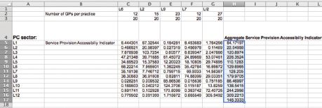
FIGURE 13.4 Service provision accessibility indicators for hypothetical medical practices in Liverpool

The level of provision per household is an indicator that divides the aggregate level of provision score by the number of households in the residence zone:

where H^im are households of different household types m. Similarly, a catchment population indicator can be calculated as

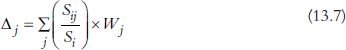
where S_i is expenditure in area i, S_ij is expenditure from area i in area j, and P_i is the population in area i. In equation (13.5), a typical term on the right-hand side involves taking the proportion of provision at j which is used by residents of i and then summing to obtain a measure of total provision for residents of i. Clarke and Wilson (1994) state that, similarly, equation (13.6) represents partitions of the residential population which are combined to form a catchment population for the centre (or outlet) at j. One can also calculate a version of this in terms of demand, which we can call ∆_j:

Other typical indicators are W_j/P_j for effectiveness and W_j/Π_j for efficiency, where W_i is the aggregate level of provision in zone i (as calculated above), P_j is the population in zone j and Π_j is the catchment of zone j. These indicators may also be disaggregated by type m (social class, car owner, etc.) and provision is disaggregated by type of good, g. The performance indicators are thus derived directly from outputs from the model to assess the levels of provision, based on the model’s predicted interaction set (Smith et al., 2006). These results may be combined with data on socio-economic status, age, ethnicity and so on. to identify areas/groups of individuals with poor access to a particular service. Thus, the key when assessing accessibility to services in rural areas is to ensure that the spatial distributions of provision and demand are such that both sets of effectiveness and efficiency indicators achieve appropriate targets.

From this example, using the service provision accessibility indicator, the access scores for residences in 12 OAs in relation to medical services were calculated for Liverpool (the highlighted column in Figure 13.4). The access scores ranged from 22.05 (indicating poor access) in L2 to 309.22 (indicating very good access), while the average access score across the 12 OAs was 148. The sixth part of accessibility analysis is the visualisation of accessibility values. Examining accessibility to services across space can be very difficult and GIS aids accessibility analysis by combining and analysing complex information from multiple sources, displaying the information in a map format. Modelling service provision in GIS can be broadly summarised under two general headings:

• the mapping of service provision in an area, region or country;

• modelling of accessibility to each service by using accessibility indicators and integrating these accessibility values into a GIS.

The development of more sophisticated GIS techniques and their widespread use among the social sciences has greatly aided accessibility analysis. Using visualisation tools, the researcher may present their results for policy analysis and evaluation. Maps can be used to display service location patterns, to provide information on where residents live in relation to service facilities, and to visualise the spatial match between service needs and resources. Indeed, previous research carried out by Halden et al. (2005) found that mapping accessibility to key services has significant advantages over analysis based on population data alone. This is because the impacts of policies taken by planners and policy-makers to increase accessibility may be seen explicitly.

Spatial interaction analysis is used in a variety of disciplines, the most prominent of which are transport, health care and retail studies. The policy emphasis on equity issues and rural accessibility has increased in recent years. Governments and regional administration centres across Europe are becoming increasing aware of the concept of spatial equity with regard to accessibility and services (European Commission, 1996, 1999). As such, policy-makers are beginning to use spatial interaction and accessibility analysis to enhance their decision-making for a number of different policy issues, including:

• assessing overall levels of expenditure and its distribution with regard to service provision (who gets what?);

• setting national and regional targets for improving equitable access to services;

• analysing local and sub-national need for services;

• examining the ex-post and forecasting the ex-ante effect of locating or relocating a service.

Conclusion

The goal of this chapter was to introduce the concept of individual-level spatial flows and how these flows can be modelled to analyse real-life events such as travel to and from medical practices. Spatial interaction analysis requires a considerable range of network and socio-economic data. Although a spatially constrained case study was presented in this chapter, calculating accessibility measures for full extents of cities, regions or countries requires a larger amount of computation, and indeed there may be trade-offs between resolution and extent of the models implemented. SIMs and the accessibility indices that may be calculated from their output provide an invaluable set of tools for describing and understanding the spatial pattern of accessibility to key services. Using information on spatial flows and accessibility indicators allows policy-makers to simulate what-if analyses using relevant transportation and socio-economic attributes. Furthermore, in conjunction with GIS, the important visual dimension to accessibility analysis can be highlighted.

FURTHER READING

Students may be interested in reading a number of follow-up books to aid their understanding of SIMs and their application. Suggested texts include: Clarke and Wilson (1994), an excellent overview of SIMs and how they are constructed; Birkin and Clarke (1991), a beginner’s introduction to spatial interaction modelling from a retail perspective; and Joseph and Phillips (1984), an excellent overview of the concept of accessibility, and why modellers should include both spatial and aspatial parameters when modelling accessibility.

Birkin, M. and Clarke, G.P. (1991) Spatial interaction in geography. Geography Review, 4: 16–24.

Clarke G.P. and Wilson A.G. (1994) A new geography of performance indicators for urban planning. In C.S. Bertuglia (ed.), Modelling the City: Performance, Policy and Planning. London: Routledge.

Joseph, A. and Phillips, D. (1984) Accessibility and Utilization: Geographical Perspectives on Health Care Delivery. London: Harper & Row.