Geocomputation: A Practical Primer (2015)

PART IV

EXPLAINING HOW THE WORLD WORKS

14

PYTHON SPATIAL ANALYSIS LIBRARY (PySAL): AN UPDATE AND ILLUSTRATION

Sergio J. Rey

Introduction

PySAL is a library for spatial analytical functions written in the open source object-oriented language Python. Since the first publication introducing PySAL (Rey and Anselin, 2007), much has transpired in the development of the library, and this chapter provides an update of this progress. PySAL was born of a collaboration between two earlier projects: PySpace and GeoDa, developed at the Spatial Analysis Laboratory at the University of Illinois at Urbana-Champaign, directed by Luc Anselin; and the STARS project, which I directed at San Diego State University (SDSU). The collaboration recognized that by pooling the efforts of the two labs, a good deal of duplication of effort could be avoided since the constituent projects were relying on a number of common core algorithms, data structures, and related modules. Rather than each group implementing the same algorithm, shared developer resources could be used to implement a single version of the algorithm for the library which each group could then leverage in their own projects. Additionally, by providing the code via a library, it now became open to a much wider user community beyond the two project groups.

In 2007, Anselin moved from Urbana to Arizona State University (ASU) to become director of the then School of Geographical Sciences and Urban Planning where he also established the GeoDa Center for Geospatial Analysis and Computation. One year later I moved from SDSU to join the faculty at ASU and become a core member of the Center. This ushered in a number of important changes in how the project was organized. First, we moved away from internal development of the code base to a more open structure by centralizing the code repository at Google Code under a BSD license. This was shortly followed by the adoption of a fixed, six-month release cycle, with the first formal release of PySAL 1.0 in July 2010. PySAL 1.8 is the current stable release, with version 1.9 set for release in January 2015.

Since the initial release of version 1.0, PySAL has been downloaded over 30,000 times, with 20,000 downloads in 2012 alone. Beyond 2012 tracking of downloads has become complicated by two developments. First, PySAL has been incorporated into the Anaconda Python Distribution,¹ which is a collection of specialized Python packages for high-performance scientific computing. Only one download of PySAL is required to build Anaconda, which in turn can be downloaded many times. The second change in PySAL’s development infrastructure was the transition of our code repository from Google Code to GitHub. Users downloading PySAL source code from GitHub are not tracked as the repositories are available for cloning and downloading by any interested party. Nevertheless, it has been gratifying to witness the growing interest in PySAL and it is timely to provide an update on the library.

The remainder of this chapter is organized as follows. The key modules that comprise the library are first described. This is followed by an overview of the different delivery mechanisms for PySAL that include interactive prompts, toolkits for GIS packages, graphical user interface (GUI) based exploratory spatial and space-time packages, high-performance computational gateways, and web services. The focus then shifts to an illustration of one particular module in PySAL: the spatial dynamics module where a selection of the analytics is applied to a case study of four decades of homicide rates for 1412 counties in the southern United States. The chapter ends with some comments about future directions for PySAL.

PySAL components

PySAL is designed as a modular library with individual components focusing on suites of analytical methods, data structures and algorithms related to a particular type of spatial or space–time analysis. Figure 14.1 provides a high-level view of the key modules in PySAL.

Spatial weights

At the core of many spatial analytical techniques is formal representation of neighbor relations between observations embedded in geographical space. There are a wealth of approaches to defining these relations and the weightsmodule implements many of the most widely used, as well as lesser known, methods. The weights module organizes these into three different classes of spatial weights:

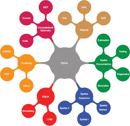
FIGURE 14.1 Pysal components

• contiguity-based weights;

• distance-based weights;

• kernel weights.

In general terms, the weights, defined as wi,j, express the potential interaction between a pair of observations i and j. In most cases the number of pairs under consideration is substantially reduced due to the specific criterion adopted which gives rise to highly sparse representations of the spatial weights.

Given their centrality in analysis, efficiencies in memory footprint and in computations involving the weights have been a high priority of our development. These efficiencies derive from heavy use of sparse matrix methods, implemented in the package SciPy (Oliphant, 2007), and allow us to scale our analytics up to large problem sizes, where ‘large’ can be on the order of several million observations in social science applications.

Interoperability has also been a guiding principle in PySAL’s development, and we have placed much emphasis on supporting a wide array of spatial weights data structures from other packages. These include read and write support for GeoDa weights, GAL, GWT, ArcGIS (Text, DBF and SWM) weights, MATLAB, GeoBugs, and STATA weights files, among others.

The weights module also has highly optimized methods for extracting topology from polygon shapefiles to generate rook- or queen-based spatial weight structures. The weights class itself has a number of useful methods such as checking for asymmetries in the neighbor relations, detection of islands (disconnected observations), and the support of various transformations on the weights including row standardization, double standardization and variance standardization.

Computational geometry

Many of the modules in PySAL make use of computational geometry algorithms, and we have centralized the latter in the computational geometry module. For example, given a set of points, the CG module supports the construction of a number of data structures, including Voronoi tessellations and minimum spanning trees, Gabriel graphs, sphere-of-influence graphs and relative-neighbor graphs. These in turn can be used by the weights module to define neighbor relations. The CG module also implements a number of efficient spatial data indices that support particular types of queries including point-in-polygon, segment intersection, projections of points onto segments and related operations.

Clustering

Methods for defining spatially constrained partitions of a set of areal units are implemented in the region module. The key approach is the max-p algorithm (Duque et al., 2012) which is a heuristic that attempts to find the maximum number of regions that satisfy some minimum floor constraint, such as the size of the population in a region or the number of areas combined, while maximizing intraregional homogeneity subject to a contiguity constraint. A key distinguishing feature of this algorithm is that the number of regions formed is endogenous, rather than having to be specified a priori by the user. In the clustering module are a set of methods to generate synthetic regions that respect the cardinality of solutions from the max-p algorithm. These provide a mechanism to evaluate the quality of the heuristic solution.

Exploratory spatial data analysis (ESDA)

Methods for global and local spatial autocorrelation analysis form the core of the ESDA module. The global methods include the analysis of binary outcomes via join count statistics with inference based on normal approximations as well as permutation-based approaches. For continuous variables, global version of Geary’s C, Moran’s I and the Getis–Ord G statistics are included, again with multiple approaches to inference. Local autocorrelation statistics include the local Moran and local indicators of spatial association (LISA) statistics (Anselin, 1995), and local versions of the Getis–Ord G statistics (Getis and Ord, 1992).

In addition to these standard measures for autocorrelation analysis, the ESDA module also includes bivariate Moran statistics as well as a suite of approaches for continuous variables that are rates, expressed as a ratio of the count of some event over a population at risk, where special care is needed due to variance instability of the attribute reflecting heterogeneity in the population at risk over the enumeration units.

Spatial dynamics

The spatial dynamics module was initially based on the space–time analytics from STARS (Rey and Janikas, 2006) but has grown with the addition of a number of newly developed methods. Three broad sets of space–time analytics are currently implemented. Markov chain-based methods, which depart from the classic discrete state Markov chain (DSMC), have been widely used in spatial analysis to model dynamics of many spatial processes including land-use change, migration, industrial structure and regional inequality dynamics among others. PySAL extends the DSMC in a number of directions to include a consideration of the role of space in shaping transition dynamics. Spatial Markov chains, first introduced by Rey (2001), allow for the influence of regional context which can introduce a form of spatial heterogeneity in the dynamics.

The spatial dynamic module also includes a LISA Markov chain (Rey and Janikas, 2006) which measures the transitions of observations across the four quadrants of the Moran scatterplot (from the ESDA module), thus extending the LISA to a dynamic context. A decomposition of the LISA Markov chain generates a pair of derived chains, one for the focal unit and one for the spatial lag, which in turn provide the basis for formal tests of the independence of the transitional dynamics for the lag and the focal chains (Rey et al., 2012). The combined use of the LISA Markov chain, together with the focal and lag marginal chains, supports the development of a rich taxonomy of space-time dynamics. Later in this chapter, I will illustrate the use of these two sets of methods.

In addition to the Markov chain-based space–time measures, this module includes several rank-based concordance measures (Rey, 2014) as well as various popular tests for space–time interaction (Knox, 1964; Jacquez, 1996).

Spatial econometrics

Modern methods of spatial econometrics are implemented in the spreg module. These include diagnostics for spatial autocorrelation in regression models based on Moran’s I (Cliff and Ord, 1981), the classic and robust versions of Lagrange multiplier (LM) statistics (Anselin and Rey, 1991; Anselin et al., 1996), and LM-based statistics for use with two-stage least squares (2SLS) residuals (Anselin and Kelejian, 1997).

Estimation methods include non-spatial ordinary least squares and 2SLS, maximum likelihood estimation of the spatial lag and error models (Ord, 1975; Anselin, 1980, 1988; Smirnov and Anselin, 2001), spatial 2SLS of the spatial lag model (Anselin, 1980, 1988), generalized moments (GM) estimation for the spatial error model (Kelejian and Prucha, 1998a), and generalized methods of moments (GMM) estimation of the autoregressive parameter in the spatial error model in the presence of heteroskedasticity as well as when endogenous variables are included in the specification (Kelejian and Prucha, 2010). GM and GMM estimation of combination models including both a spatial lag term and a spatial autoregressive term are included (Kelejian and Prucha, 1998b; Arraiz et al., 2010; Drukker et al., 2013). Finally, a family of spatial regime specifications is supported which incorporate spatial heterogeneity for all included estimation methods with Chow tests for spatial coefficient heterogeneity (Anselin, 1990).

In addition to state of the art estimation methods, spreg includes an array of non-spatial diagnostics, including a multicollinearity condition number, Jarque–Bera test for normality and tests for heteroskedasticity including Breusch–Pagen, Koenker–Basset and White’s test. The spreg module supports the use of a rich set of spatial weights including various contiguity criteria, distance bands, k nearest neighbors and inverse distance as well as kernel-based weights required by the heteroskedasticity and autocorrelation consistent estimators, and the module handles non-spatial endogenous variables.

Other PySAL modules

There are several additional PySAL modules not portrayed in Figure 14.1. The inequality module includes the classic Gini and Theil inequality indices as well as spatially explicit versions of these that can be used to analyze interregional inequality. These include decomposition-based statistics for Theil along with approaches to inference (Rey, 2004) as well as a spatial Gini index (Rey and Smith, 2013).

PySAL also includes a number of so-called ‘contributed’ modules. These are not part of the core library itself, but rely on optional dependencies that a user may have installed for particular types of analyses. Contributed modules currently exist for Shapely (Gillies et al., 2008) and a visualization module which supports choropleth mapping through matplotlib (Hunter, 2007). The latter will be demonstrated in the empirical illustration below.

PySAL use cases

By design PySAL as a library is intended to support a variety of delivery mechanisms and use cases. This is a recognition of the diversity of end users and of computing platforms that spatial analytical services are consumed on. Below I outline the different use cases supported by PySAL.

Interactive computing

In many areas of scientific investigation, often one does not have a clear hypothesis in mind and instead adopts an exploratory, or data-driven, approach to the analysis. Here the use of an interactive prompt is invaluable as the ultimate scientific workflow is not readily apparent, and instead the next computational task that the research will apply is only known after the results of the previous step are generated. PySAL supports interactive computing using either the built-in Python interpreter or the more powerful IPython shell (Pérez and Granger, 2007).

Graphical user interface clients

A second use case that PySAL supports is the wrapping of components of the library in rich desktop clients which provide access to the underlying functionality through a user-friendly GUI. One such example is the package Crime Analytics for Space–Time (CAST). Figure 14.2 shows one selected CAST window which is illustrative of the kind of functionality it supports. CAST enables the joint consideration of multiple types of spatial supports (polygon, point, network) in a powerful and flexible set of fully interactive dynamic graphics. Also shown are calendar maps that provide insights into the temporal distribution of crime events.

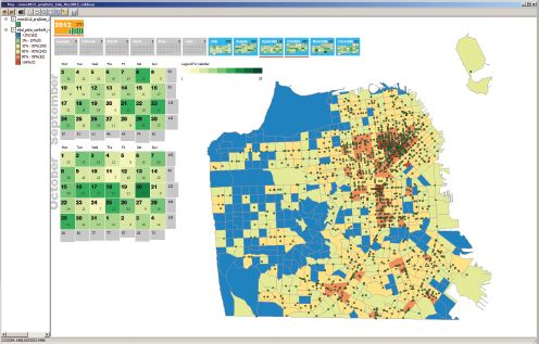
FIGURE 14.2 Crime Analytics for Space–Time (CAST)

The specialized nature of CAST is emblematic of a development philosophy at the Center where end user applications are tightly focused on the spatial analytical functionality most appropriate to a substantive problem domain, in this case the spatial dynamics module. Rather than attempting to develop a one-size-fits-all GUI-based application, the wide scope of methods in the PySAL engine can be selected from to develop tailored applications in a time-efficient manner.

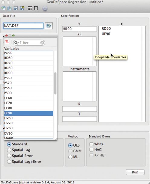
FIGURE 14.3 GeoDaspace model specification dialog

Another prominent example of a standalone application built around a PySAL core is the GeoDaSpace package, which is based on the wxPython module for its graphics and provides the end user with easy access to the advanced functionality in the spreg module. GeoDaSpace shields the user from many of the low-level operational and technical implementations while focusing on the most common operations and options. An example of one of the model specification dialogs for GeoDaSpace is shown in Figure 14.3.

GIS toolkits

In addition to interactive shells and GUI clients, users can interface with PySAL through toolkit architectures of geographic information systems (GIS) such as ArcGIS and QGIS (see O’Brien, Chapter 17). Figure 14.4 displays an example of an early version of a toolbox for ArcGIS 10.1.²

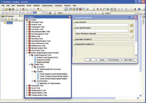
FIGURE 14.4 ArcGis PySal toolbox

Web services

A final delivery mechanism for PySAL is through web services. These make a selection of the spatial analytic functionality available to the end user via a browser. An example is CGPySAL, which can be seen in Figure 14.5. This provides an interface to spreg on the CyberGIS Gateway (Wang, 2010). Here the user can upload their own data and then, using a flexible drag-and-drop interface, select variables to specify a model.³

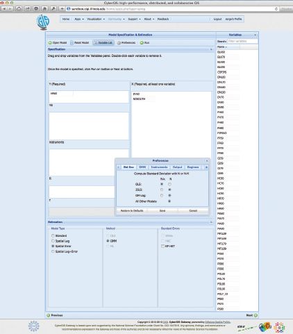
FIGURE 14.5 CGPySal spatial regression in the CyberGIS Gateway

In addition to enabling distributed computing whereby endusers no longer require local installation of software, the centralized installation of PySAL as part of the CyberGIS Gateway allows us to implement a highly optimized version of PySAL that fully exploits the characteristic of the underlying hardware. This results in computational gains that are generally not available in the version of PySAL that is released for users to install locally since we focus on general portability in that version rather than targeting specific hardware.

Illustration

Given the scope of the modules in PySAL, space limitations prevent an exhaustive set of illustrations. Instead I focus on one particular module, spatial dynamics, and a case study exploring the dynamics of homicide patterns in 1412 southern US counties using data developed as part of an earlier broader project (Baller et al., 2001; Messner et al., 1999). The focus here is on illustrating the use of PySAL with an empirical dataset. A detailed substantive investigation is beyond the scope of this chapter.

Spatial distribution of homicide rates

Figure 14.6 shows choropleth maps for the homicide rate (HR = homicides per 100,000) using a quintile classification for the decades 1960–1990. The classification method is one of the options in the PySAL map classification module and it is used here with the contributed visualization module mentioned previously.

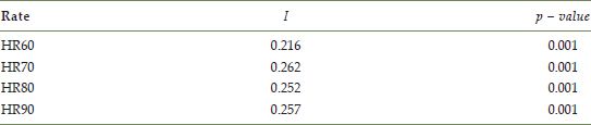
Examination of the class boundaries indicates that the lower four quintiles are fairly stable over the four decades, while the fifth quintile is highest in the first decade (92.94), drops in the intermediate two decades, and then rises up to 64.26 in 1990. An aspatial view of the distribution dynamics is portrayed in Figure 14.7 which suggests that the overall level of homicide was actually lower in the first and last decade, relative to the middle two decades, if the medians are considered. At the same time, applying Moran’s I to the homicide rate for each decade reveals significant positive spatial autocorrelation in all periods (Table 14.1).⁴

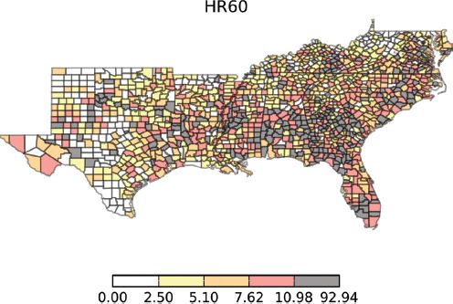
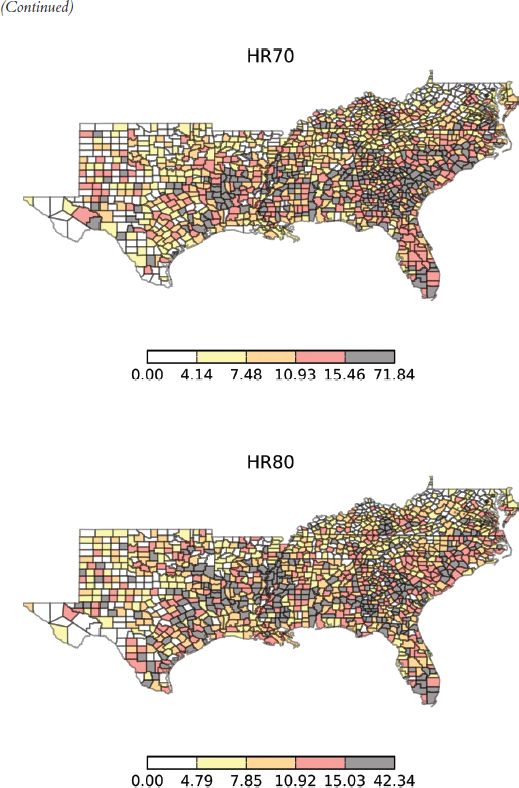
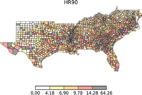
FIGURE 14.6 Homicide rate, 1960–1990: (a) 1960; (b) 1970; (c) 2980; (d) 1990

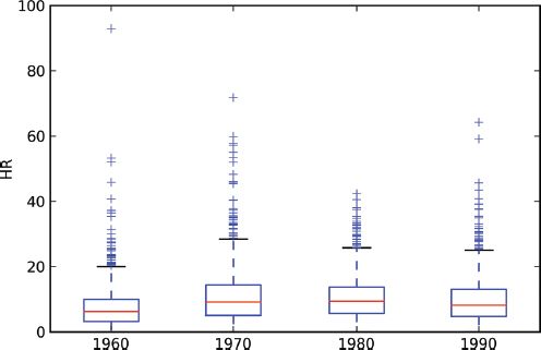
FIGURE 14.7 Boxplots of homicide rate, 1960–1990

TABLE 14.1 Moran’s I (queen contiguity) for homicide rate, 1960–1990

Spatial distributional dynamics

The global measures of autocorrelation are similar over this period, suggesting that the pattern of homicide activity may be relatively stable. Similarly, the stability of the majority of the quintiles may also be interpreted as evidence of distributional stability. However, both sets of measures are global, or whole map, measures that may mask more complex dynamics at work within the distribution. PySAL’s spatial dynamic module has a number of space–time analytics that consider the role of space in the evolution of distributions over time.

Discrete Markov chains

The first of these is based on a classic discrete Markov chain which uses the quintiles to define the states of the chain. More specifically, the homicide rate in each county is viewed as a sample chain that can take one of five discrete values corresponding to its position in the quintile distribution in a given year. By pooling all the sample chains, the probability transition matrix can be estimated via maximum likelihood as

where ni,j,t is the number of times a sample chain started in state i in period t and transitioned to state j in the next period. Applying this estimator to our sample chains gives the estimated transition probability matrix P in Table 14.2.

TABLE 14.2 Homicide rate transition probabilities

There is strong evidence of mobility in the homicide rate distribution as the probability of remaining in the same quintile over sequential decades is less than 0.50 for all quintiles. The mobility is higher for the intermediate quintiles than is the case for the first and last quintiles. Lower mobility for the fifth class is to be expected given the skewed nature of the homicide rate distribution in each decade which results in a wider interval for that state in the Markov chain. Interval width alone, however, does not account for the lower mobility in the first quintile as its width is similar to that of the fourth quintile.

The last row in Table 14.2 is the estimated long-run steady-state distribution π, which suggests a uniform distribution holds when the chain reaches equilibrium. Note that although the states of the chain are defined using the quintiles of the distribution, this does not imply that the ergodic distribution will necessarily be uniform. In other words, there is no evidence of a convergence of homicide rates in particular parts of the distribution in the long run.

Spatial Markov chains

The classic discrete Markov chain provides a first view of the distributional dynamics; however, it does not consider the spatial location of the sample chains and how the local context of a county might affect the chain’s movement in the distribution and transitions across states. One approach to this is the spatial Markov chain which conditions the transition dynamics of a county’s homicide rate on the spatial lag of homicide rates. In other words, rather than a single transition probability matrix P, counties may face a different transition matrix depending on their spatial context.

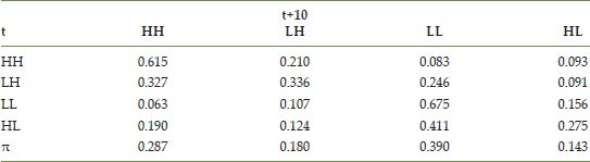
Use of the spatial Markov class in PySAL estimates the conditional transition probability matrices reported in Table 14.3. The matrices are ordered according to the value of a chain’s spatial lag at the beginning of the transition period, so that the first conditional matrix P (1) is for chains that had neighbors with homicide rates in the lowest quintile, and the last matrix P (5) is for chains with spatially lagged homicide rates falling in the upper quintile. These are estimated using

where n(l)i,j,t is the number of times a sample chain with a spatial lag in quintile l started in state i in period t and transitioned to state j in the next period.

TABLE 14.3 Spatially conditioned transition probability matrices

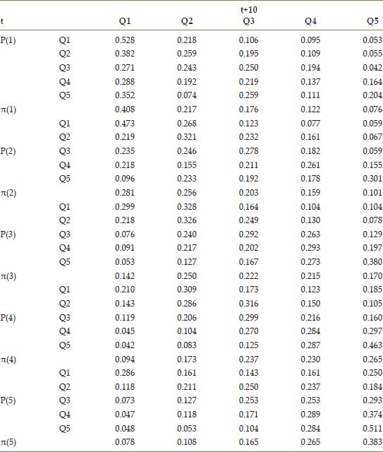
Examination of the table reveals that the spatial context of a chain can influence its transition dynamics over a decade. Counties that have homicide rates in the fifth quintile face different probabilities of remaining in that quintile depending on whether their surrounding counties also have rates in the upper quintile (p(5)5,5 = 0.511), or if the neighbors fall in the fourth quintile (p(4)5,5 = 0.463). At the other end of the spectrum, counties with the lowest homicide rates face a higher probability of remaining in the first quintile when their neighbors are also in the first quintile (p(1)1,1 = 0.528) relative to when the neighbors’ rate falls in the second quintile (p(2)1,1 = 0.473). A formal test for the heterogeneity of the transition probabilities across lag quintiles rejects the null (H₀: P=P(l) for all l={1,2,…,k}) of a single homogeneous transition probability matrix .

The spatial heterogeneity in the transition probabilities also has implications for the estimated long-run distribution of homicide rates. Recall that under the homogeneity assumption, the long-run distribution is uniform across the five classes. By contrast, there are five separate estimated conditional ergodic distributions in Table 14.3, none of which are uniform. The mass of the distribution moves towards the tail of the distribution reflected in the value of the conditional lag – for example, the distribution conditioned on the first lag quintile π(1) is right skewed, while the distribution conditioned on the fifth lag quintile π(5) is left skewed. Moreover, the long-run distribution conditioned on the central lag quintile π(3) departs from uniformity as the mass moves out of both tails and into the central three classes.

LISA Markov chains

The spatial Markov chain provides insight into the role of regional context at the beginning of a transition period in influencing the movement of a county’s homicide rate within the distribution over time. In other words, different spatial contexts display different distributional dynamics. Those conditional dynamics, however, generate new realizations of the spatial lag for each county in the next period, and the question of how the county’s homicide rate may co-evolve with its spatial lag naturally arises.

The spatial dynamics module includes several analytics designed to address this question. One way to visualize the co-movement of a county’s homicide rate with that of its spatial lag is to consider the origin standardized movement vector (Rey et al., 2011) obtained from comparing Moran scatterplots (Anselin, 1996) from sequential decades. Figure 14.8 pools all the movement vectors over the three transitions (1960–1970, 1970–1980, 1980–1990), which provides an impression of the directional tendencies in the distributional dynamics. One striking feature is the relative asymmetry of the lengths of the movement vectors when considering the focal unit dimension (x-axis) versus the spatial lag dimension (y-axis). This is due to the spatial lag operator being a weighted average of homicide rates, whereas for the focal unit only the raw rate is considered. Thus the latter will tend to have variances that are greater than or equal to those of the lag.

It is important to note that the movement vectors reflect relative movement of a LISA within two scatterplots, and not absolute movements. In other words, movements to the southwest in Figure 14.8 indicate a county’s homicide rate was declining in concert with a decline in value for its spatial lag. Similarly, movements to the northeast represent increases in the focal county’s homicide rate and that found in its neighboring counties between two periods. These do not necessarily represents movements between quadrants in the Moran scatterplot.

Here we slightly abuse the notion of an ‘absolute move’ to define it as a movement across one of the four quadrants of the Moran scatterplot. From this, we can define a LISA Markov chain where the states of the chain are taken as the four quadrants of a Moran scatterplot in a given period (HH = 1, LH = 2, LL = 3, HL = 4), where HL indicates that the crime rate in the county was above the average for that period while its spatial was below average. Between any two decades a county’s position in the Moran scatterplot may change to transition between the quadrants. Collecting all these transitions allows for the estimation of LISA Markov transition probabilities reported in Table 14.4.

Examination of these probabilities reveals several interesting characteristics about the spatial dynamics of homicide rates. First, the staying probabilities (i.e, probability of remaining in one state of the space) are highest for quadrants 1 (HH) and 3 (LL) of the scatterplot. This is indicative of relative stability in positive spatial autocorrelation that we encountered in the application of the global Moran’s I statistic earlier. Second, the estimated equilibrium distribution for the LISA chain is to have the mass of the distribution more concentrated in these two classes (amounting for almost two-thirds of the distribution), again reflecting the dominant pattern of spatial clustering.

A third pattern seen in Table 14.4 is that when movements out of a quadrant do occur they are more likely to reflect the contribution of the movement of the homicide rate in the focal county than they are the movement of the spatial lag. For example, considering the chains in the initial state HH, the movement to LH, which involves an absolute change for the focal unit rate but not the spatial lag, occurs more frequently than movement to HL, which involves a change in the absolute position of the lag but not the focal rate.

Similarly, for an initial state of LL, moves to HL are more frequent than moves to LH. These patterns reflect the asymmetry in the magnitudes of the movement vectors in Figure 14.8 alluded to previously.⁵

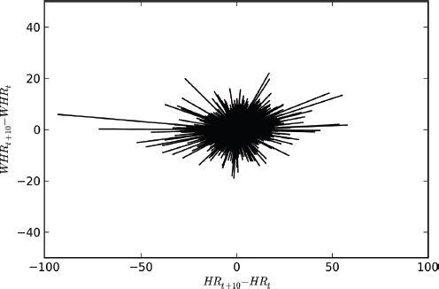
FIGURE 14.8 Origin standardized LISA movement vectors for homicide rates

TABLE 14.4 LISA Markov transition probabilities

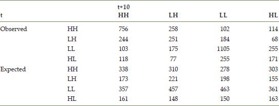
A formal test for co-movement dependence can be derived by decomposing the LISA chain into two marginal chains, one for the focal unit (i.e. the own chain O) and one for the lag chain (i.e. for the neighbors N). Each of these marginal chains has two states, H for high and L for low, relative to the mean value in a given period. Under the null that these two chains are independent the expected transition probability matrix for the joint chain (i.e., the LISA chain) is given by

where is the Kronecker product operator, P(O) is the transition probability matrix for homicide rates, and P(N) is the transition probability matrix for the spatial lag of homicide rates. Table 14.5 reports the observed and expected joint spatial chain transitions. A formal test of the difference between these two estimated transition probability matrices resulted in , indicating the movement of a county’s homicide rate in the distribution is not independent of the movement of homicide rates in neighboring counties.

TABLE 14.5 Observed versus expected joint spatial chain transitions

Summary

Application of PySAL’s spatial dynamics module to the case of homicide data has revealed clear evidence of spatial contextual effects in shaping the evolution of homicide activity distributions over space and time. At the same time it is important to keep in mind that the patterns identified are indirect evidence of spatial diffusion processes and do not imply a particular causal structure. The latter requires confirmatory modeling that reflects specific structural mechanisms giving rise to the patterns identified here. Nevertheless, detection of the patterns via the application of exploratory space–time methods suggests that such investigation is warranted.

Conclusion

This chapter has presented an update, overview, and illustration of the Python Spatial Analysis Library. Given the scope of the modules contained in PySAL, the illustration focused by necessity on only a subset of the analytical functionality provided by the library, but this should serve to provide the reader with a flavor of how PySAL can be used in practice.

One of the strengths of open source spatial analysis projects is that through the efforts of development teams, new state-of-the-art methods appearing in the scientific literature are often implemented in libraries that serve an important dissemination function. In this regard, PySAL shares in this effort, yet a unique feature of the PySAL project is that several of the core developers have also been the creators of new spatial analytical methods that then become components of the library. By building on the contributions of others, this has allowed us to focus on the parts of the spatial analytical research stack where our efforts can have the most impact.

PySAL is well situated to contribute to an evolving CyberGIS infrastructure, and several ongoing projects are focused on embedding PySAL in high-performance environments. The notion of spatial analytical workflows requires frameworks for tracking the provenance of a sequence of analytical operations that are chained together to produce a result. We are currently exploring a prototype of such a provenance framework that captures the workflow in a distributed context and would support full replication of results. Closely related to this work is the development of a spatial econometrics workbench (Anselin and Rey, 2012) that would target spatial econometrics in particular but bring the methods from the spreg module of PySAL into a distributed application available to researchers to access through web browsers.

Finally, it is important to mention that our targeting of the Python language and scientific community is sometimes questioned by spatial scientists who are more familiar with R and the ecosystem of associated spatial packages, as the implication is that we are diverting energies that should otherwise be directed towards R. While we understand the sentiment behind such questions, we think they are somewhat misplaced for several reasons. Firstly, at the time of PySAL’s conception, Python was beginning to make major inroads into scientific computing, yet spatial analysis was largely absent. We felt that focusing on Python would serve an important dissemination mechanism whereby leading developments in spatial analysis could be brought to new communities. The inclusion of PySAL in Anaconda is evidence that we have achieved some success in this regard. Secondly, we do not see our efforts as duplicative of the excellent work in R-related projects. Moreover, with new tools like the IPython notebook, it is now possible to use R and PySAL together in the same workflow. From this perspective, developments in either project R or PySAL can serve to benefit the other.

FURTHER READING

PySAL has extensive documentation available for both end users as well as developers. See http://pysal.org for full details.

ACKNOWLEDGEMENTS

Recent development of PySAL has been supported by Award No. 2009-SQ-B9-K101 from the National Institute of Justice, Office of Justice Programs and National Science Foundation Grant OCI–1047916.

¹http://docs.continuum.io/anaconda/pkgs.html.

²At the time of writing the ArcGIS toolbox is in alpha, with a stable release planned for spring 2015.

³The main site for CGPySAL is https://sandbox.cigi.illinois.edu/home/.

⁴The global results are robust to the choice of the spatial weights matrix (rook versus queen).

⁵The LISA Markov chain also has options for conditioning on the significance of the static LISA in each period of the transition. These are not reported here due to space limitations.