Geocomputation: A Practical Primer (2015)
PART IV
EXPLAINING HOW THE WORLD WORKS
15
REPRODUCIBLE RESEARCH: CONCEPTS, TECHNIQUES AND ISSUES
Chris Brunsdon and Alex Singleton
Reproducibility in research
The term reproducible research (Clærbout, 1992) has appeared in the scientific literature for nearly two decades (at the time of this writing) and has gained attention in a wide range of fields such as statistics (Buckheit and Donoho, 1995; Gentleman and Temple Lang, 2004), econometrics (Koenker, 1996) and signal processing (Barni et al., 2007). The aim of reproducible research is that full details of any results reported and the methods used to obtain these results should be made available, so that others following the same methods can obtain identical results. Clearly, this proposition is more practical in some areas of study than others – it would not be a trivial task to reproduce the chain of events leading to samples of lunar rock being obtained, for example! However, in the area of geocomputation, and particularly spatial data analysis, it is a reasonable goal.
To some, the justification of reproducible research may be self-evident. It may even be seen as a necessary condition for well-founded scientific research. However, if a more concrete argument is required, perhaps the following scenarios could be considered:
1. You have a data set that you would like to analyse using the same technique as described in a paper recently published by another researcher in your area. In that paper the technique is outlined in prose form, but no explicit algorithm is given. Although you have access to the data used in the paper, and have attempted to re-create the technique, you are unable to reproduce the results reported there.
2. You published a paper five years ago in which an analytical technique was applied to a dataset. You now discover an alternative method of analysis, and wish to compare the results.
3. A particular form of analysis was reported in a paper; subsequently it was discovered that one software package offered an implementation of this method that contained errors. You wish to check whether this affects the findings in the paper.
4. A dataset used in a reported analysis was subsequently found to contain rogue data, and has now been corrected. You wish to update the analysis with the newer version of the data.
Each of the above scenarios (and several others) describe situations that cannot be resolved unless explicit details of data and computational methods used when the initial work was carried out are available. A number of situations may arise in which this is not the case. Again, some possibilities are listed:
1. You do not have access to the dataset used in the original analysis, as it is confidential.
2. The dataset used in the original study is not confidential, but is available for a fee, and you do not already own it.
3. The dataset used in the original study is freely available, but the original study does not state the source precisely, or provide a copy.
4. The steps used in the computation are not explicitly stated.
5. The steps used in the computation are explicitly stated, but require software that is not free, and that you do not already own.
6. The steps used in the computation are explicitly stated, but the software required is not open source, so that certain details of procedures carried out are not available.
Addressing the problems
All of the situations above stand in the way of reproducible research. In situation 1 this state of affairs is inevitable unless the researcher interested in reproducing the results obtains consent to access the data. Situations 2 and 5 can be resolved by financial outlay if sufficient funds are available, but situations 3, 4 and 6 cannot be resolved in this way. For this last set of situations, it is argued that resolution is achieved if the author(s) adopt certain practices at the time the research is executed and reported. Situation 6 is in some ways a variant of situation 4 where non-disclosure of computational details is due to a third party rather than the author of the research, and can be resolved if, whenever possible, open source software is used.1
However, attention in this discussion is focused on situations 3 and 4. Both of these situations arise if exact details are not made widely available. In most cases, this is not done with malice aforethought on the part of researchers – few journals insist that such precise details are provided. Although, in general, researchers must cite the sources of secondary data, such citations often consist of acknowledgement of the agency that supplied the data, possibly with a link to a general website, rather than an explicit link (or links) to a file (or files) that contained the actual data used in the research. Similarly, the situation described earlier in which computational processes are described verbally rather than in a more precise algorithmic form is often considered acceptable for publication.
Software barriers to reproducibilty
Another source of uncertainty in identifying exact data sources or code used is that this information is not necessarily organised by the researchers in a way that enables complete recall. Typically this occurs when software used to carry out the analysis is interactive – to carry out an analysis a number of menu items were chosen, buttons clicked and so on, before producing a table or a graph that was cut and pasted into a word-processing document. Unfortunately, although interactive software is easier to use, its output is less reproducible. Some months after the original analysis it may be difficult to recall exactly which options were chosen when the analysis took place. Cutting and pasting the results into another document essentially broke the link between the analysis itself and the reporting of that analysis – the final document shows the output but says nothing about how it was obtained.
In general, unless interactive software has a recording facility, where commands associated with mouse clicks are saved in some format, and can be replayed in order, then graphical user interfaces and reproducible research do not go well together. However, even when analysis is carried out using scripts, reproducibility cannot be guaranteed. For example, on returning to a long-completed project, one may find a number of script files with similar content ‒ but no information about which one was actually run to reproduce the reported results ‒ or indeed, whether a combination of ‘chunks’ of code from several different files were pasted into a command-line interface to obtain reported results.
Literate programming
To address these problems, one approach proposed is that of literate programming (Knuth, 1984). Originally, this was intended as a means of improving the documentation of programs – a single file (originally called a WEB file) containing the program documentation and the actual code is used to generate both a human-readable document (via a program called Weave) and computer readable content (via a program called Tangle) to be fed to a compiler or interpreter. The original intention was that the human-readable output provided a description of the design of the program (and also neatly printed listings of the code), offering a richer explanation of the program’s function than conventional comment statements. However, WEB files can also be used in a slightly different way, where rather than describing the code, the human-readable output reports the results of data analysis performed by the incorporated code. In this way, information about both the reporting and the processing can be contained in a single document. In this case, rather than a more traditional programming language (e.g. Pascal or C++), the code could be scripts in a language designed specifically for data processing and analysis, such as R or SAS. Also, the Weave part of the process could also incorporate output from the data processing into the human-readable part of the document.
Examples of this approach are the NOWEB system (Ramsey, 1994) and the Sweave package (Leisch, 2002). The former incorporates code into LATEX documents using two very simple extensions to the markup language. The latter is an extended implementation of this system using R as the language for the embedded code.
An example of Sweave
This chapter was created using Sweave, and the simple example of analysis of variance in Table 15.1 was created with some incorporated code.
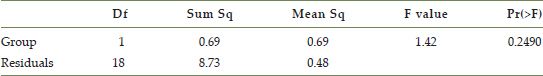
In this case, the code is echoed in the document, and the result is incorporated in the final document. A number of other options are possible ‒ for example, the code need not be echoed, and the output can be interpreted directly as LATEX code, giving the output in Table 15.2.
Note that from the echoed code, this document contains information about the data (via assignments to the variables ctl, trt, Group and Weight) as well as the steps used to analyse the data. If this document is passed to a third party, they will be able to reproduce the analysis by applying the Sweave program. Also, by using a further program, Stangle, they will be able to extract the R code.
TABLE 15.1 R ANOVA: example of incorporated code
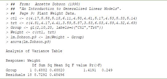
TABLE 15.2 Formatted ANOVA output
A geocomputation example
The previous example demonstrates the general principle of Sweave but does not involve geographical data. The choropleth map in Figure 15.1 is produced using the GISTools package. This demonstrates not only the use of spatial data, but also that the system is capable of including graphical output from the incorporated code. As before, the R commands are echoed to the document to illustrate the method, although in more usual situations this would not be the case.
The previous example showed a reproducible exercise in standard map creation in R. Figure 15.2 shows the result of applying pycnophylatic interpolation (Tobler, 1979) to another variable from the 1990 US Census. Here the variable considered is the number of children aged one year and under, on a per-county basis. This variable is obtained from the same source as the previous example. Pycnophylactic interpolation is a technique used to estimate population density as a continuous surface, given a list of population counts for a set of supplied corresponding geographic zones. Here, the population counts are numbers of children aged under one year old, and the zone boundaries are obtained from the shapefile used in the previous example. The surface approximation is designed to be smooth in terms of minimising roughness R defined by
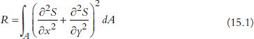
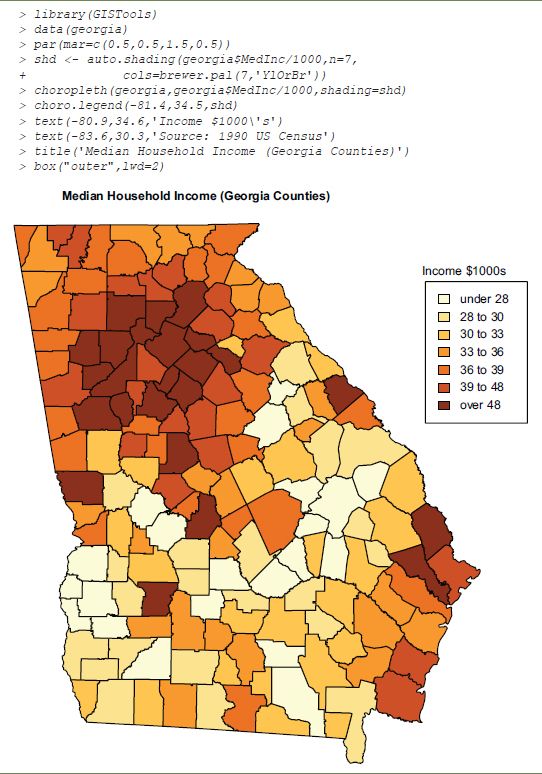
FIGURE 15.1 Incorporated R code producing graphical output
Source: 1990 US Census
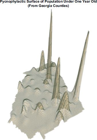
FIGURE 15.2 Incorporated R code producing graphical output: pycnophylactic surface
Source: 1990 US Census
where A is the geographical region under study and S is the density, a function of location (x,y), subject to the constraints that the integrated population totals over the supplied set of zones agree with the empirical counts provided. In practice this is achieved using a finite element approximation, so that population counts for small rectangular pixels are computed. These calculations are carried out using the R package pycno (Brunsdon, 2011).
In the example, graphical output from the code is used once again, although this time a three-dimensional surface is shown rather than a conventional map.
Implications for geocomputation
The above example demonstrates the incorporation of documentation, analysis and data in a single document. However, the example was not geographical. The key question here is how practical is this kind of approach in a geocomputation context. A number of issues arise:
1. Geocomputational data sets can sometimes be large, or in other ways impractical to reproduce.
2. Geocomputational computation times can be large.
3. Can combinations of text and code be expressed in other formats than R and ![]() ?
?
The first two of these are perhaps harder to address. In the example here the data consists of around 20 numbers, but in many situations the data is much larger than this, and it becomes impractical to incorporate the data in a WEB type file. One approach may be to incorporate code that reads from a specific file – although ultimately this still implies that code and data must be distributed together to allow reproducible research. An alternative might be to provide details (such as URLs) of where the data were downloaded – for instance, by incorporating code used to obtain the data if R was used to access data directly from a URL. However, in this case reproducibility depends on the remote data not being modified.
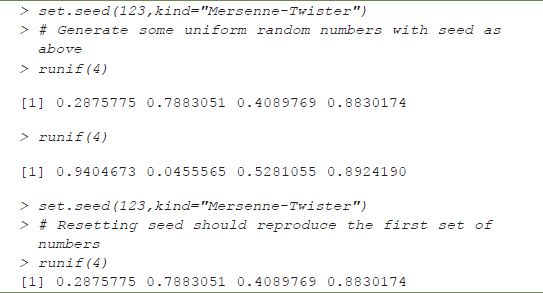
The second problem is not so much one of reproducibility, but one of practicality. Some simulation-based approaches (and other methods using large datasets) may require code taking several hours to run, and therefore major resources are required for reproduction; this is a scaled-down version of the ‘lunar rock’ example in the introduction. Reproduction may therefore be difficult, but not impossible; this is simply in the nature of such research. Another issue with simulation-based studies is the use of random numbers – unless the software being used gives explicit control of the generation method and specification of a seed, distinct runs of the same code will give different results. Fortunately, in R such control is possible (see Table 15.3); however, this is not possible in Microsoft Excel, for example.
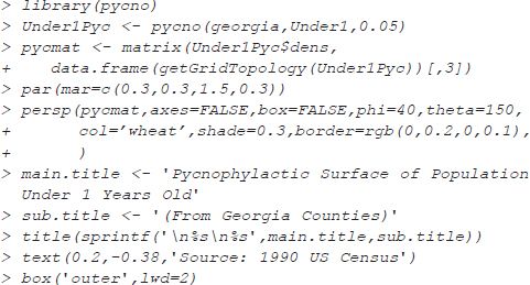
TABLE 15.3 Demonstration of seed control in R
The final issue listed is the use of alternative formats for either the text or code in literate documents. This is of key practical importance for the GIS community, many of whom do not typically use either LATEX or R. If reproducibility is as fundamental a concept as is being argued here, then ideally an inclusive approach should be adopted – simply insisting that all geographical information practitioners learn new software is unlikely to encourage uptake. A further literate programming tool, StatWeave (Lenth, 2012), offers more flexibility, allowing a number of different programming languages and statistics packages to be embedded into LATEX, including SAS, Maple, STATA and flavours of Unix shells. Unfortunately at this stage, there are is no GIS software embedded in this way, although StatWeave does offer the facility to incorporate new ‘engines’ into its portfolio, so that other command-line-based software tools can be used. A number of possibilities exist here ‒ for example, incorporating Python would allow much of the functionality of either ArcGIS or QGIS to be incorporated. Also, returning to Sweave, there are a number of R packages for handling geographical information.
For others, a bigger barrier to adopting either Sweave or StatWeave is the use of LATEX as a typesetting tool, when they are more accustomed to a word processor. However, it is possible to use StatWeave to process .odf files (the XML-based format for OpenOffice files) with embedded code, and there is an R package, odfweave, offering the same functionality (provided the embedded language is R). In both cases, the embedded code is typed directly into a document, which is then saved and post-processed to replace the embedded code with the output that it generates in a new .odf file. OpenOffice is then capable of saving the files into .doc or .docx formats, although obviously it is important to distribute the original .odf files with embedded code if the documentation is to be reproducible.
The difficulty for some is perhaps a move away from a GUI-based cut-and-paste approach to producing documents. Unfortunately, in its current from this approach is the hardest to reproduce, as was stated earlier. There are some possible future developments that could address this, however. If, when images or tables were cut and pasted, the object contained information about the process that created it (perhaps by journalling a set of Python or other commands recording a user’s interaction with the GUI), then these could be embedded in a document (e.g. an .odf file), although this would require a more fundamental redesign of existing GIS software.
However, the adoption of such practices offers major advantages:
• It is helpful for authors who can reproduce figures and calculations in the revisions of a paper or report.
• It is helpful to others who want to carry out research in the field can work from the current state of the art, without having to ‘reverse engineer’ algorithms and techniques.
• It provides a framework for verification if the methods used in a given paper or report are called into doubt.
Although the adoption of these practices may require a little initial effort, the above factors suggest that the long-term payback easily justifies this.
FURTHER READING
As well as the items in the References, there are a number of very useful websites that discuss reproducible research. A few of these are listed below:
• http://adv-r.had.co.nz/Reproducibility.html provides some useful tips for carrying out reproducible research in R.
• http://blog.stodden.net/category/reproducible-research/ is Victoria Stodden’s blog about reproducible research.
• http://reproducibleresearch.net/blog/ is a very comprehensive link site for work on reproducibility.
1The distinction is made here between open source software such as that discussed in O’Brien, Chapter 17, where the source code is distributed regardless of whether there is a distribution fee; and zero cost software, which is obtained without fee, but may not have openly available source code.
All materials on the site are licensed Creative Commons Attribution-Sharealike 3.0 Unported CC BY-SA 3.0 & GNU Free Documentation License (GFDL)
If you are the copyright holder of any material contained on our site and intend to remove it, please contact our site administrator for approval.
© 2016-2026 All site design rights belong to S.Y.A.