Geocomputation: A Practical Primer (2015)
PART V
ENABLING INTERACTIONS
17
OPEN SOURCE GIS SOFTWARE
Oliver O’Brien
Introduction
This chapter reviews some of the most popular software packages in the well-developed and wide-ranging open source GIS software field. This is not intended to be a comprehensive review, as this is already well covered (Steiniger and Bocher, 2009; Donnelly, 2010; Tsou and Smith, 2011; Steiniger and Hunter, 2013). It should be borne in mind that, as with all actively developing software fields, and in particular those where open source has a strong contribution, such as GIS, the literature can quickly be superseded by developments.
Open source GIS software has a long history, but is also currently rapidly evolving. For example, Geographic Resources Analysis Support System (GRASS: http://grass.osgeo.org/), one of the earliest open source GIS software packages, was initially released in 1984; by contrast, QGIS (http://qgis.org/), another GIS software package, is much more recent, and its development is becoming increasingly active. Furthermore, in some sense, modern GIS software is increasingly difficult to define, and in addition to traditional desktop-based software packages such as GRASS or QGIS, there are web map servers, such as MapServer (http://mapserver.org/) and GeoServer (http://geoserver.org/), along with geospatial web (geoweb) client libraries to display spatial data online. Furthermore, a plethora of GIS functions for the storage, manipulation or analysis of spatial data are incorporated in other classes of open source software such as spatial databases or statistical programming languages such as R (http://r-project.org/). There are also various library packages, often coupled to many GIS and other applications, and specialist tools aimed at solving specific problems. The website http://opensourcegis.org now lists over 300 applications and libraries.
What is GIS software?
Geographic information systems (GIS) software allows the storage, simultaneous display, analysis and visualisation of multiple pieces of geographic information. Figure 17.1 shows a typical three-step software workflow between GIS data sources, GIS software and the final presentation of the content. Core desktop GIS software capabilities are, however, increasingly divergent, for example, with the addition of new functionality related to the end-presentation of geographic information. For example, by including functionality enabling enhanced cartographic styling and adornments of maps, these encapsulate a role that was traditionally carried out by conventional (non-georeferenced) graphics programs.
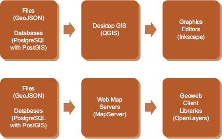
FIGURE 17.1 Typical GIS software flows. Top: Desktop-based GIS workflow for map production. Bottom: Server/Client GIS workflow for web display of geospatial information. Examples in brackets
Furthermore, some databases now implement spatial analysis functionality directly, which can be useful when volumes of data are very large, and subsumes the analytical functions that may traditionally have been completed within a desktop GIS package. For example, the PostGIS (http://postgis.net/) extensions to the PostgreSQL (http://www.postgresql.org/) open source database can carry out a wide range of spatial operations.
What is open source software?
Software can be considered to be open source if it is distributed with its source code files, and with a licence that allows the free use, adaptation and redistribution of the source code. Users can examine the code to understand it, and potentially enhance it. The licence is often carried forward, so that if enhancements are made and distributed, the licence applies to them as well. Open source software is also typically (but not exclusively) made available for free. Copyright often remains with the creator, and attribution to the original and subsequent authors of the code may have to be retained. There are numerous variants of open source software licences. Popular examples include the Berkeley Software Distribution (BSD) licence, which simply asserts copyright and allows redistribution and use of the software as long as the creator is attributed (but not used to promote the software), and the General Public License (GPL), which ensures that modified versions of the software will always remain open for further modification and free use.
A key benefit of having access to source code means that if a limitation or problem is encountered, a user with the appropriate skills can examine the underlying source code, either to understand why it is behaving the way it is, or even to fix an issue or adapt it. The results of such corrections can then be shared with the user community. A wide pool of developers, with many different backgrounds, abilities and resources, can help improve a project by approaching problems in different ways, improving the overall quality by collaboration, consensus and visibility – the principle of ‘many eyes’. An important body within the open source software field is the Open Source Initiative (http://opensource.org/) which considers open source software to be software distributed without the traditional copyright restrictions, where source code is included and can be viewed and adapted.
The open source GIS community
Many open source GIS packages have come from academic institutions and public bodies seeking to address a specific need. As their software has continued to evolve, a worldwide community has been built up to take on, manage and promote such projects. The Open Source Geospatial Foundation (OSGeo) is the principal organisation that promotes and organises the major open source GIS projects around the world. It has a number of established projects, and also an ‘incubator’ where smaller but promising projects are built up. Most of the software packages outlined in this chapter come under the auspices of OSGeo. OSGeo produces a DVD, OSGeo Live, that contains all its software projects together in one place, suitable for trying out. The DVD can be created from disk images at http://live.osgeo.org/.
OSGeo also organises an annual conference, Free and Open Source Software for GIS (FOSS4G). The conference takes place at locations around the world and typically has up to 1000 participants. It is often used to launch new versions of open source GIS software projects. For example, in the 2013 conference in Nottingham, UK, major software launches and announcements included QGIS 2, GeoServer 2.4, the first beta of OpenLayers 3 and OSGeo Live 7.
A further organisation, Open Geospatial Consortium (OGC), is concerned primarily with defining standards for spatial data formats. Such standards are generally widely supported within open source GIS software, either natively or often through the GDAL library, an OSGeo project which acts as a translation layer between many geospatial formats, including those defined by the OGC. Some of the well-known standards that have been defined by the OGC include KML (originally from Google Earth) which describes layers and viewpoints and annotations when looking at a map, Web Map Service (WMS) which is a standard way of requesting and presenting map images, and Styled Layer Descriptor (SLD) which is a format for defining how to represent features cartographically.
Desktop GIS
Desktop GIS software is a key interface for moderate and expert users to expose geospatial data to investigation, analysis and visualisation. The two most prominent open source desktop GIS software are GRASS and QGIS.
GRASS was originally developed by the US Army and is over 30 years old; it is now a core project administered by OSGeo. GRASS is a command-line application, but has a graphical user interface (GUI) called wxGUI. In addition, GRASS functionality has been linked into QGIS. GRASS contains a huge number of modules, which have a particular naming convention – for instance, modules that perform vector operations start with a ‘v.’. For example, v.hull takes a vector map and produces a corresponding convex hull polygon. By contrast, r.slope.aspect creates slope and aspect raster maps from an elevation map. As GRASS is natively operated from the command line, it has a relatively steep learning curve for those unfamiliar with operating a GIS. More information on GRASS can be found at the project’s website (http://grass.osgeo.org/).
QGIS, formerly also known as Quantum GIS, is an open source desktop GIS, designed from the start to be easy to use and cross-platform. It has a large and active community of developers, whose activities have recently accelerated, as it builds out its core features and becomes more widely adopted by the desktop GIS-using community. It is tightly integrated with the Python scripting language and PostGIS database servers; and versions are available for various operating systems. QGIS includes many standard spatial analysis functions (contained with a package formerly called SEXTANTE but recently renamed Processing) and can also integrate with a GRASS installation, thus allowing access to the many GRASS modules from within QGIS. QGIS can read from and write to a wide variety of spatial file and database formats. To access many of the formats, QGIS uses ogr2ogr, part of the GDAL library of tools.
The QGIS user interface design consists of a main window showing the mapping data, with a reorderable and togglable layer list. Operations are carried out using menus or one of numerous toolbars. A separate Print Composer window can be used to place the layered and styled map on a virtual sheet of paper, and adornments can be added. The resulting map can then be saved as a vector PDF, SVG or a number of other formats. The Print Composer is intended to replace the traditional final step of producing a map from GIS data where a graphics editor may be used.
The extensibility of QGIS has led to a number of complementary projects, including QGIS Cloud (a geodata infrastructure service), QGIS Server (allowing views of QGIS maps and layers to be accessed by multiple users) and a QGIS for Android project, bringing the application to a major mobile device ecosystem. The application itself can be driven through an API, making custom versions of QGIS with specific features and workflows branded and streamlined. The availability of the API also has enabled an array of plugin extensions to be created. For example, the Time Manager plugin, by Anita Graser, allows temporal geodata to be easily viewed in the application, using a time slider (Figure 17.2). Further information on Time Manager can be found at http://anitagraser.com/projects/time-manager/.
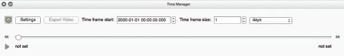
FIGURE 17.2 Time slider in the Time Manager plugin in QGIS
There are numerous other open source desktop GIS applications, which are similar to GRASS or QGIS, but typically present alternative user interfaces or different feature emphasis, such as concentrating on raster/field operations. For example, uDig (http://udig.refractions.net/) is a Java-based desktop GIS that shares QGIS’s goals of being user-friendly and multiformat. gvSIG (http://www.gvsig.org/) is another Java-based desktop GIS that, like QGIS, uses the SEXTANTE package for spatial analysis. GeoDa (https://geodacenter.asu.edu/ogeoda) specialises in sophisticated exploratory spatial data analysis, autocorrelation and modelling of point and polygon data, looking at the links between spatial and non-spatial statistics of the data. Opticks (http://opticks.org/) focuses more on processing and analysing remote sensing and imagery data. Both gvSIG and Opticks have the status of being incubator projects within OSGeo.
Spatial databases
Storing geospatial data effectively and efficiently has always been a key aspect of open source GIS, particularly as the two- or three-dimensionally varying nature of geographical information means that data volume can become extremely large. While flat file formats, such as Shapefile or GeoJSON, are good for storing some geospatial data, a dedicated database server can often be necessary. Typically, the ability to manage or analyse spatial data is provided by extensions to traditional relational database servers (RDBMS). For example, MySQL (http://www.mysql.com/) is an open source RDBMS and is part of the ‘LAMP’ (Linux Apache, MySQL, PHP) software stack that is widely used for simple dynamic webpages. However, core MySQL has been extended with spatial functions, enabling the storage of spatial data classes, alongside analytical functions.
Perhaps the most established and actively developed open source spatial database is PostgreSQL, with the PostGIS extension. PostgreSQL is a general purpose open source relational database server that was first released in 1986. PostGIS is a more recent package of stored procedures, definitions and extensions that enhances PostgreSQL by allowing it to deal with spatial structures, defined through special geometry and geography data types. The server was known for its complex installation and configuration process, particularly relating to memory requirements, and while care is still needed to install and specify a server that will perform optimally for the type and use of data stored within it, it is now more functional ‘out of the box’.
Mapnik, an open source graphical renderer for maps, can use PostGIS-enhanced PostgreSQL databases as data sources. An appropriate query for certain features is defined by the programmer, and Mapnik modifies the query by adding spatial parameters. In the following example SQL query, the section in italics has been specified by the programmer, and Mapnik wraps additional SQL around it to capture the data for only a particular area. 900913 is a spatial reference ID (SRID) for the coordinate reference system (CRS) that the bounding box is specified for. PostGIS stored procedures generally have an ‘ST_’ prefix.
SELECT ST_AsBinary("geom") AS geom, "metric" FROM (select geom, gid, geographycode as name, QS606EW0048/(QS606EW0001*1.0) as metric from c11_ew_oa_bfe_augm_google as b, c11_ew_oa as d where d.geographycode = b.oa11cd and QS606EW0001 > 0) as foo WHERE "geom" && ST_SetSRID('BOX3D(-46473.71319738716 6684876.745708373,-22013.86414613076 6709336.594759629)'::box3d, 900913)
PostGIS/PostgreSQL databases can also be added as data sources to QGIS, and a further extension to PostgreSQL, called pgRouting (http://pgrouting.org/), can be accessed through QGIS by using the PgRouting Layer plugin. pgRouting allows PostgreSQL/PostGIS to be used for complex routing queries over any topologically connected network of any kind, such as the UK’s mainline railway network and other metro networks available in OpenStreetMap (Singleton, 2014a).
Web map servers
Web map servers access layers of geospatial content from databases and files, and serve them to web clients, either as simple HTML for display without further processing by standard web browsers, or in a format that can be handled by JavaScript (or similar) ‘geoweb’ client libraries such as OpenLayers, viewed within the web browser. They generally use one of two standards specified by the OGC – WMS (raster images) or Web Feature Service (WFS: geospatial objects as vectors). WMTS is a variant of WMS that serves WMS data in standardised square tiles, that can, if necessary, be pre-rendered for speed. TMS and XYZ are alternative specifications for naming and structuring sets of tiled map images, they share somes similarity to WTMS but are simpler to use. Web map servers are not always required in a typical map-based website toolchain, as web clients can do limited file processing, database access (via a simple proxy) and layering. Similarly, web map servers do not necessarily require a geoweb client library, as they can pre-render, annotate and deliver maps as images that can be displayed in a web browser using simple HTML.
There are two major open source web map servers, MapServer (http://mapserver.org/) and GeoServer (http://geoserver.org/), both of which are OSGeo projects. MapServer is a long-standing project, written in C, that allows users to browse GIS data and web application developers to create geographic image maps that direct users to content. It supports many standards for geographic data, and various vector and raster data formats. It is frequently used to provide WMS mapping images and was originally developed in conjunction with NASA, to make its satellite imagery more easily accessible. GeoServer is a Java-based server that, like MapServer, can process and display mapping data to a wide variety of standards and in many formats. It can work with various Java Servlet containers.
Geoweb client libraries
Geoweb client libraries are typically JavaScript-based pieces of software that are loaded into a user’s web browser when they visit a website that includes an interactive map, allowing that map to be displayed with layers, augmented and navigated by the user. Web map servers can deliver simple images to a web browser with no geoweb client libraries needed; however, use of a geoweb client library allows the user much more flexibility to pan/zoom around a map, request additional function and view vector data, feature pop-ups and so on. The first popular ‘modern’ geoweb client library was the Google Maps API. Although not open source, and with its access limited to API calls rather than deep integration with client code, it gave access for web map developers to Google’s extensive, and free, mapping and aerial imagery, while allowing the maps to be easily augmented with vector features – the famous ‘red pins’ being the simplest example. The service initially did not have any usage or load restrictions. Allowing anyone to augment a map in such a simple way, without requiring a dedicated service with a web map server on it, worrying about the cost, or needing much in the way of programming or installation knowledge, meant the service became hugely popular and inspired a number of open source peers.
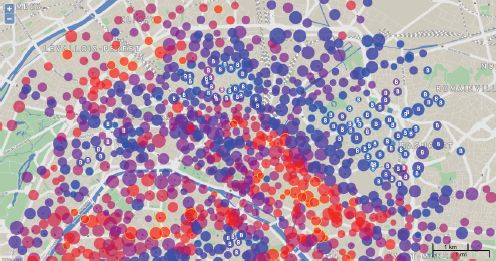
FIGURE 17.3 Example of an OpenLayers 2 map, showing styled vector data as circles of various sizes, colours, border highlights and labels. Two Openlayers adornments, a zoom control and an automatic scale bar, are included. The background map is copyright OpenStreetMap contributors
OpenLayers (http://openlayers.org/) is perhaps the oldest and best established open source geoweb client library. It was for many years used to power the default rendering of the OpenStreetMap project, as shown at http://www.openstreetmap.org/, although that recently switched to an alterative library, Leaflet (http://leafletjs.com/). OpenLayers 3 was recently released, although the widely deployed version 2 (http://openlayers.org/two/) remains available for download. There are significant differences in functionality between the two versions and both are likely to remain key geoweb client libraries for a while. This new version of the library is a major rewrite, which aims to simplify the object structure, and ease adoption of the library, which can have a steep learning curve. OpenLayers can read in numerous formats, including WMS, GeoJSON and Shapefile, as well as TMS and XYZ map tiles used on Google Maps, Bing Maps, and other sources. The library, being pure JavaScript, is easily installed on a web server and hooked into webpages via a simple call to load the JavaScript. The OpenLayers website includes annotated examples, wiki-based general documentation and JavaScript API generated documentation. One of the strongest features of OpenLayers is its advanced vector styling capabilities (Figure 17.3). This includes rule-based styling, allowing vector symbols to have varying colours, opacities, label display and orientation. OpenLayers partially implements the SLD specification from the OGC.
Leaflet, shown in Figure 17.4, is a more recent JavaScript geoweb client library. It shares many of the same features as OpenLayers and has similar default functionality, displaying maps in a draggable or ‘slippy’ pan/zoom manner with a minimal user interface (by default) of a pair of zoom buttons. However, it was written from scratch to present a straightforward implementation of ‘slippy maps’ for developers. It also, from the beginning, focused on mobile web applications, dealing well with touch-based (as well as mouse-based) interaction, although OpenLayers has also more recently included this as core functionality. It is very lightweight, requiring a download by the viewer of just 33 kb of compressed and minified JavaScript code. The small code size means it does less ‘out of the box’ but has a plugin architecture to incorporate additional file formats and other layer types. For example, TileLayer.GeoJSON implements support for the increasingly popular GeoJSON spatial file format, while Leaflet.GeoSearch allows a Leaflet-based map to easily integrate with a number of third-party geocoding services such as Google’s.
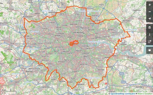
FIGURE 17.4 Example of the Leaflet geoweb client library, here presenting a rendering of OpenStreetMap data that appears on the project’s main website. Highlighted as vectors are the Greater London and City of London boundaries, and a nominal location for the ‘London’ label
Other open source GIS software
This section has only touched upon of the huge variety of open source GIS software, many fulfilling particular aspects of a geospatial toolchain. One key software technology not covered so far is R (Cheshire and Lovelace, Chapter 1). This scripting language has its roots in the academic/scientific community, as a powerful and comprehensive mechanism for performing statistical analyses programmatically, but its open source status and design, together with its ease of manipulating data in sophisticated structures (such as matrices), has allowed it to find many uses. A large and active community have developed geospatial-specific functions for R, many of which are contained in the sp package maintained by Roger Bivand.
One final package of note is Routino (http://www.routino.org/). This is a routeing software package that is specifically geared to using OpenStreetMap data for routeing. The software can be run as a website, or from the command line, and can be used to easily and quickly generate routes across the road and path network for a parcel of OpenStreetMap data that is converted to a format suitable for fast processing. Different traffic profiles can be specified, such as obeying one-way directions on particular road segments, using steps, maximum speeds and road type desirabilities, and detailed route descriptions can be created.
Applying open source GIS
The following section illustrates how to create an informational map of rail transport accessibility in London with the QGIS open source GIS application, integrating freely available (and open) spatial data sources. The intention is to identify those built-up areas in the city that are not well served by railway or metro stations.
Because the area is within Great Britain, we take advantage of the Ordnance Survey Open Data datasets (http://www.ordnancesurvey.co.uk/opendatadownload/). The Ordnance Survey is the institutional mapping agency for the country. Its datasets can be considered to be generally complete and authoritative, and certainly sufficient for this task. The following data are needed for this task: the administrative boundary of London; the extent of built-up areas within the city; and the location of railway and metro (e.g. London Underground) stations.
The following datasets need to be downloaded from the Ordnance Survey, they are generally large files (40–400 MB):
• Boundary-Line – from which the London boundary can be derived. At the time of writing, the name of the file when downloading is bdline_gb.zip.
• Ordnance Survey Strategi – which includes data on urban extent. At the time of writing, the name of the file when downloading is strtgi_essh_gb.zip.
• Ordnance Survey VectorMap District (vector version) – for myriads TQ and TL. From this data, railway/metro stations can be obtained. At the time of writing, the names of the two files when downloading are vmdvec_tq.zip and vmdvec_tl.zip.
These datasets can be obtained directly from the Ordnance Survey webpage referenced above, but may also be downloaded from the MySociety mirror at http://parlvid.mysociety.org:81/os/ which does not require registering and waiting for an email link to the data. Ordnance Survey data in Great Britain is split up into a grid of 100 km × 100 km squares, known as myriads, which are assigned a sequential two-letter code. The TQ myriad covers almost all of London, but TL is also needed for completeness, covering a small section in the far north of the city, which has some building development and a single station, Crews Hill.
You can install QGIS by downloading it from http://qgis.org/ and following the installation instructions. Depending on your version of QGIS, the following instructions and screenshots may vary slightly.
Loading spatial data layers into QGIS
Before loading in the required data, change the project projection to British National Grid – choose Project Properties from the Project menu, select Enable ‘on the fly’ CRS transformation, type ‘British National Grid’ into the Filter box, select the resulting item and press OK. This sets up the map projection for the map, as shown in Figure 17.5.
Choose Add Vector Layer from the Layer menu. Navigate to the uncompressed bdline_essh_gb folder, then under the Data subfolder, choose greater_london_const_region.shp.
Choose Add Vector Layer from the Layer menu. Navigate to the uncompressed strtgi_essh_gb folder, then under the data subfolder, choose urban_region.shp.
Choose Add Vector Layer from the Layer menu. Navigate to the uncompressed OS VectorMap District (ESRI Shape File) TQ folder, then under the data subfolder, choose TQ_RailwayStation.shp. Repeat this step for the TL folder.
QGIS should now look like Figure 17.6 – note that the colours used to display each layer are randomly picked so will be different if the steps above are followed. Because the boundary layer was added first, the QGIS window will have zoomed to its extent. You may need to alter the colour of the railway station dots so that they stand out from the building outlines sufficiently – this can be done by right-clicking on the layer in the layer list on the left, choosing Properties from the pop-up menu, then Style and then Color.
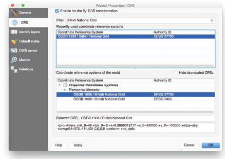
FIGURE 17.5 Setting the project’s coordinate reference system
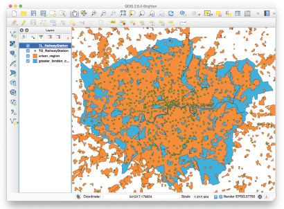
FIGURE 17.6 The Layers loaded into QGIS
Preparing the data for analysis
We are focused on the area of London, so we need to prepare layers to show only this extent. First we need to create a polygon containing the simple administrative boundary of London. We carry this out by performing a Dissolve operation. Under the Vector menu, choose Geoprocessing Tools, then Dissolve. Make sure the correct layer is selected, choose FILE_NAME as the attribute to dissolve by (as it is the same for all the polygons in the layer) and choose an appropriate name for the new file. Tick the ‘add the result to canvas’ checkbox, so that the new layer is added straight in to QGIS. Finally, you can delete the old layer by right-clicking on it in the list and choosing Remove. See Figure 17.7.

FIGURE 17.7 Preparing the data: The Dissolve operation
We then need to clip the other three layers to this new layer just containing a London polygon. This is done using the Clip operation which is under the Geoprocessing Tools. Be sure to select the new London boundary layer as the layer to clip to. You need to repeat this step for all three of the other layers. Each time, you can remove the original layer after you add the new layer. This is shown in Figure 17.8.
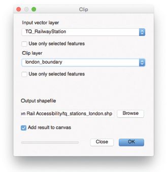
FIGURE 17.8 Preparing the data: the Clip operation
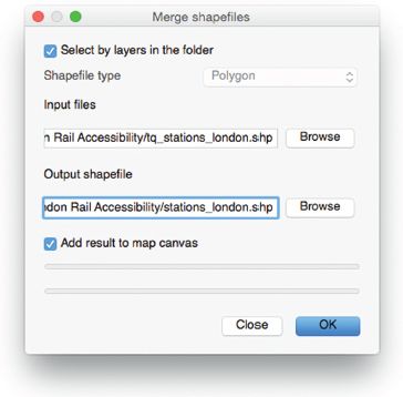
FIGURE 17.9 Preparing the data: merging shapefiles
Finally, we want to merge the TL and TQ layers together. This will reduce the four layers to three. This is done in a similar way to the above – but using the Data Management Tools submenu and then the Merge shapefiles to one menu item (Figure 17.9).
On completion of these spatial operations, the window should look something like Figure 17.10.
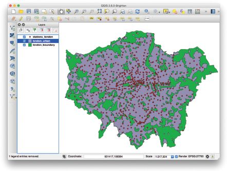
FIGURE 17.10 The merged map
Performing spatial analysis on the data
We want to show built-up areas (i.e. those with significant concentrations of buildings) that are far from railway stations. We define such areas as those that are further than 1 mile (approximately 1610m), in a straight line, from any station.
We do this in two steps. First, we add a one-mile buffer around the stations. This is done by the Buffer option, in the Geoprocessing Tools submenu. The Buffer distance should be set to 1610 as our projection (British National Grid) has units in (real) metres. Add the new layer to the map as normal and tick Dissolve buffer results. The result is shown in Figure 17.11. Finally, we subtract the buffer from the urban area layer. To do this, choose Difference from the Geoprocessing Tools submenu. The input layer is the urban area layer, clipped for London. The difference layer is the new buffered stations layer. The resulting layer is once again added to the list of layers, and all others, apart from the London boundary, can be removed. See Figure 17.12.
It is necessary to name the areas identified. To do this, add in another layer from the Strategi data – settlement_seed.shp. Clip this to the areas layer that was created, then edit the properties for the resulting clipped labels layer, by right-clicking and choosing Properties. Choose Labels, tick Label this layer with and choose NAME. Add some appropriate styling – for example, a 1mm buffer is recommended as this will make the text stand out more from the background. Figures 17.13–17.15 show this sequence.
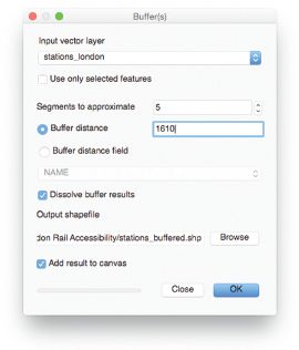
FIGURE 17.11 Performing the spatial analysis: adding a buffer
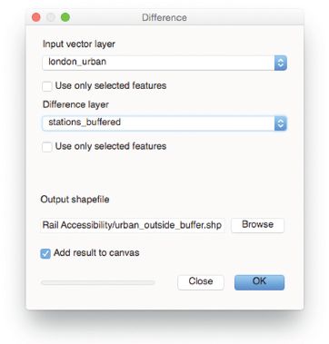
FIGURE 17.12 Performing the spatial analysis: subtracting the buffer from the urban area layer
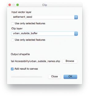
FIGURE 17.13 Naming the areas: Clip operation
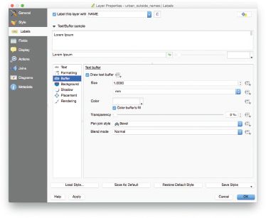
FIGURE 17.14 Naming the areas: editing layer properties
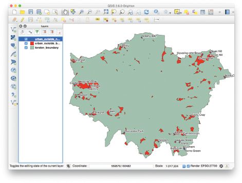
FIGURE 17.15 Naming the areas: adding some styling
Creating a map
Our analysis has been performed, and labels have been added. Now we just need to produce the final map. Choose New Print Composer from the Project menu and specify an appropriate name. Choose Add Map from the Layout menu and drag out an area for the main map, leaving some space around the edges of the virtual sheet of paper for adornments. In order to ensure that the full London area is shown, you may need to go to the Item properties tab, then click on the Set to map canvas extent button. See Figure 17.16.
Finally, you can add in adornments, such as a scale bar or a title. These are again accessed under the Layout menu, then by dragging each item onto the map. Options are displayed in the Item properties tab on the right of the Print Composer. When you are happy, you can generate a PDF, SVG or other formats, with the Export menu items on the Composer menu. Both PDFs (Figure 17.17) and SVGs generated from this map will be saved as vectors, so will print to a high quality.
Conclusion
This chapter has illustrated some of the main categories of open source GIS software, and community infrastructure supporting its development, promotion and use.
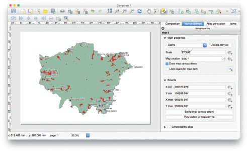
FIGURE 17.16 The Print Composer
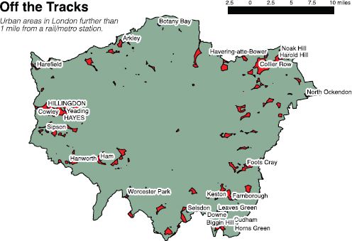
FIGURE 17.17 The final map saved in PDF format
An example of spatial analysis of transport accessibility is given using QGIS to demonstrate how open source GIS can be utilised in an applied context. It is just one task possible with using just one of many open source GIS software packages. It is fair to say that open source GIS can perform just about any geospatial operation it is possible to do – and the extensibility associated with open source software means that it is extremely easy for programmers to enhance their preferred open source GIS toolchain to perform a novel task at hand.
While it is generally the case that established and traditional commercial GIS software packages in the market have a support, documentation and training structure that open source solutions may not yet match, this is countered by the speed of development and insight that open source allows and promotes. Open source GIS software in its own right has developed business opportunities. Some companies, such as Mapbox, manage various projects and provide a hosting and configuration option for those who do not wish to learn the toolchain themselves. Effectively, the service of delivering the product is commercialised rather than the product itself. Additionally, the core developers of some the most active open source GIS projects may provide consulting services or contracted development of custom features. In this way, both commercial and community end-users benefit from the accelerated improvement in the space.
FURTHER READING
Books and online documentation for open source GIS software are invaluable as a reference for understanding the software and becoming familiar with its structure and usage. There are a range of good books on many of the applications mentioned in this chapter, published by Packt Publishing, and available as eBooks or as physical printed books. For example:
• Corti, P., Mather, S.V., Kraft, T.J. and Park, B. (2014) PostGIS Cookbook. Birmingham: Packt Publishing.
• Graser, A. (2013) Learning QGIS 2.0. Birmingham: Packt Publishing.
• Gratier, T., Hazzard, E. and Spencer, P. (2015) OpenLayers 3 Beginner’s Guide. Birmingham: Packt Publishing.
• Iacovella, S. and Younglood, B. (2013) GeoServer Beginner’s Guide. Birmingham: Packt Publishing.
As with all well-used and modern open source software, there is also a wealth of information available on the web.
All materials on the site are licensed Creative Commons Attribution-Sharealike 3.0 Unported CC BY-SA 3.0 & GNU Free Documentation License (GFDL)
If you are the copyright holder of any material contained on our site and intend to remove it, please contact our site administrator for approval.
© 2016-2026 All site design rights belong to S.Y.A.