Geocomputation: A Practical Primer (2015)
PART I
DESCRIBING HOW THE WORLD LOOKS
2
GEOGRAPHICAL AGENTS IN THREE DIMENSIONS
Paul M. Torrens
Introduction
At their foundation, geographical agent-based models (ABMs, see Crooks, Chapter 4) are spatial processors, tasked with collecting and organizing geographic data, relating it to geographical concepts, animating it relative to space–time conditions, and adding contextual value in the meantime. Most geographical ABMs are automata (Turing, 1936; von Neumann, 1951) and follow in the distinguished tradition of finite-state (Minsky, 1967) and intelligent machines (Turing, 1950). As automata, ABMs are highly flexible in their ability to achieve any requirements put to them in computation. One common use of ABMs is in representing geographical things in simulation, and these things could be information, people, cities, biology, cars, snowflakes, and so on. Indeed, much of the appeal of ABMs is a by-product of their flexibility in representing and handling geographical entities, processes, and phenomena, and ABMs have been usefully employed in modeling a range of geographical systems, in public health, urban studies, landscape dynamics, medicine, economics, and other areas.
While they boast considerable inherent and implied extensibility, many geographical ABMs limit their scope to two dimensions of space in practical applications, which often puts them at odds with the realities of systems that they are tasked with modeling. The reasoning for constraining ABMs to two-dimensional spaces is varied, but in short, the addition of a third spatial dimension adds considerable complexity in model-building and simulation, invoking some long-standing challenges in computing three-dimensional spatial processes atop conventional GIS infrastructures. Overcoming the difficulty of adding dimensionality to geographical ABMs could substantially broaden the range of applications to which ABMs could be put, and it could expand their utility in supporting applied geocomputation.
In this chapter, I will review some of the complications that present in building three-dimensional space–time agency and related representations, and I will introduce a novel variation on ABMs – polyspatial agents – as a vehicle for addressing those challenges. I will discuss the usefulness of polyspatial agents with reference to simulating human interaction in crowds and earthquake scenarios, where dimensionality is critical to building authentic models, and where the requirements for space–time geocomputation are rather unforgiving for traditional GIS and ABMs.
Why agents need a third dimension of space
When considering a third dimension for geographical ABMs, it is important to assert that this encompasses shifting the theory, representation, applications, processes, data infrastructure, and computing of agents into an immersive volumetric space, which is a departure from traditional representation of agents on half-planes or similar two-dimensional manifolds. The potential advantages (and dilemma) of adding a third dimension to geographical ABMs are wide-reaching, but the focus here is on those of particular saliency for geocomputation: characterization, geographic information, sense and sensing, interaction, and meta-simulation.
Characterization
In many application scenarios, agents are characters, and the peculiarities of this characterization are important to the function that they play within the scenario. Characterization affords agents particular attributes, traits, constraints, and tendencies, determining whether (and how) they might be economically motivated (Tesfatsion, 1997), rational (Arthur, 1994), maximizing (Simon, 1956), evolutionary (Holland, 1995), and so on. Agent characteristics also play a (starring, supporting, or bit-part) role in how the dynamics of a system play out, and how agents’ individual roles contribute to larger ensembles is critical in assessing the aggregate (i.e. group, population, regional, network, component) characteristics of the system (Janelle et al., 1998; Lee et al., 2007; Parrish and Hamner, 1997; Raafat et al., 2009; Reynolds, 1999; Schmidt and Griffin, 2007; Shaw et al., 1999). This may include system interaction (Doxiadis, 1968; El-Shakhs, 1972), dependencies (Krugman, 2005), complexity (Batty, 2005), allometry (Batty, 2008), and related collective traits for physical, mechanical, biological, chemical, or informational agency. The characterization of the environments that house and support agents is also important, as this provides the substrate for much of their agency. For geographical agents, the ambient environment often supplies a significant source of their geographic information (Golledge and Stimson, 1997).
It is therefore important that agents are afforded three-dimensional characteristics when that level of dimensionality is relevant to the role that they are cast in. However, most characteristics of geographical ABMs are represented in one or two dimensions of space, and in many cases this limits their functionality in simulation. Consider some examples. The locomotion of walking agents’ bodies is often reduced to vectors cast from artificial centroids of simple point masses (Helbing and Molnár, 1995). In geographical ABMs, urban buildings and streetscapes are usually reduced to two-dimensional polygons (Haklay et al., 2001) or network geometries (Gayle et al., 2009). When terrain is considered in geographical ABMs, it is commonly tessellated and abstracted into an affordance value (Guy et al., 2010). These reduced characterizations are convenient – particularly when ABMs need to be coupled with GIS – but they are also artificially restrictive relative to the real-world systems that modelers could represent in simulation.
Geographic information
Reduced dimensionality is quite prevalent in ABMs that rely on geographic information systems (Zlatanova et al., 2002) and spatial data models (Abdul-Rahman and Pilouk, 2008) designed for such systems, in part because GIS has been relatively slow to embrace three dimensions due to lingering technical challenges (Goodchild, 2009).
The usual approach to handling three dimensions of space in a GIS (and in ABMs) is to constrain the system to a 2-manifold and infer a third dimension as data values ascribed to objects on the 2-manifold (we can think of this as 2.5-dimensionality). Yet, fully three dimensions of geographic information are critical in understanding and representing a host of systems of interest to geocomputation, and for facilitating geocomputational operators and analyses. By placing agents – and the objects and entities that they might interact with – in a volumetric dimension, one can generate a variety of spatial information that is inaccessible from two-dimensional manifolds (up/down, surmountability, packing and space-filling, shadowing, pitch and roll, morphology of concave (and some convex) polyhedra, 3-manifold structure, etc.). One may also produce more nuanced information about projected two-dimensional conditions by considering a third geometrical dimension (rather than a simple attribute value), and this holds for elevation, relief, collision, visibility, line of sight, occlusion, coverage, parallax, hierarchy, traversability, shape, pose, degrees of freedom, displacement, and so on.
Sense (and sensing) of space and place
Our perception and awareness of environments (as humans or as other objects and entities) is also often informed by three dimensions of space. Many aspects of space and place, for example, simply make little sense on planar representations, such as the shortest path through a multi-story building with stairs (Ferguson and Stentz, 2007) or underwater trajectories (Petres et al., 2007; Ware et al., 2006). Our everyday experiences with sensing ambient geographic information rely on the third dimension, particularly if we must negotiate barriers with ambulatory difficulty (Church and Marston, 2003), for example. The need for a third dimension also translates into the user experience of communicating and working with simulations. In some cases, it may be convenient to reduce the dimensionality of a simulation’s output to two dimensions, but in other cases an immersive experience is desirable, and this in part explains the recent popularity of virtual worlds (Bainbridge, 2007; Crooks et al., 2009; Delaney, 2000; Economist, 2006) and digital globes (Butler, 2006; Goodchild et al., 2012) in geographic information science. Indeed, the third dimension is likely to become even more important as geographical ABMs move to augmented reality platforms (Feiner et al., 1997; Uricchio, 2011).
Yet, representation of agents’ sense of surroundings is often two-dimensional, and this is evident in collision detection routines, synthetic vision, and even economic geography. On the latter point: think about how we usually consider distance decay (Alonso, 1967; Clark and Evans, 1954), for example, and how little sense a two-dimensional (really one-dimensional in the case of bid-rent profiles: Brown and Holmes, 1971) distance decay and friction parameter makes for a real estate market like Hong Kong, which hosts a majority of multi-level structures. To some extent, developments in three-dimensional sensing of geographic information have reinforced the primacy of two-dimensionality, and this is evident for LiDAR (Gamba and Houshmand, 2002), in particular, where height measurements are sampled along a two-dimensional plane, missing overhangs and casting a “melted wax” appearance to many urban environments.
Interaction
It is when we consider interactions of and among things in space and time that denying ourselves a third dimension of space really starts to seem like a shortcut. Touching, brushing, smashing, breaking, separating, covering, fleeing, aligning: these are all interactions that necessitate three-dimensional representation to be treated realistically. This is especially true when we consider physical processes among rigid-body objects, particularly on the surface of the Earth, where gravity and friction are crucial in explaining the dynamic of interactions, but other properties between objects also require a third dimension, particularly for soft-body interactions (deformation, elasticity). For human agents, the approximation of movement relative to geographic planes is often problematic when mapped to two dimensions: while walking, for example, people use their feet to contact the ground for acceleration, stopping, rotation, and turning (Winter, 2009), and their center of gravity is a dynamic function of the ambulation of their body and limbs; these details are often reduced to simple point-mass representations (Bouvier et al., 1997; Schweitzer, 1997) or cylindrical extrusions (van den Berg et al., 2008) in geographical ABMs, with the result that well-known artifacts are produced when they interact (Torrens et al., 2012).
Meta-modeling and multi-modeling
Docking – exchange of algorithms and data – between geographical ABMs and other models and simulations is also a challenge in dimensionality. Even though many geographical ABMs are content to sit on two dimensions of space, the models (and model systems) that we often would like them to interact with are treated in three dimensions. For geographical ABMs to participate in meta-model systems (models of models) or multi-models (where the results from one model provide dynamics to another), higher-dimensional data must often be abstracted if they are to have parity. In essence, we must jettison significant detail to allow geographical ABMs to ‘talk’ to other models that work with higher dimensions, and this is evident in connections between geographical ABMs and voxelized community climate models, many CAD-based building information models, Earth science models that treat sub-surface Earth processes, models of gaseous flow (Epstein et al., 2008), and so on.
Existing approaches
Significant effort is being devoted to changing how the community addresses these challenges, and there are many existing implementations of geographical ABMs that adopt three dimensions of space. This is, for example, a prominent topic of research in the biology community, where ABMs of cell formations are used to explore dynamic formation of neoplasms (Malleta and De Pillis, 2006), or the dynamics of organ structures such as the epidermis (Chapa et al., 2013). There is also agent-based work on movement of entities within biological systems (Burkitt et al., 2011).
In physical geography, automata-based models (of which we can consider agent automata a variant), particularly cellular automata, are popularly used to enhance traditional gridded and lattice models (Malamud and Turcotte, 2000; Rothman and Keller, 1988) or continuum models of particle movement (Avolio et al., 2000; Baxter and Behringer, 1990; Iovine et al., 2003; Kronholm and Birkeland, 2005), and three-dimensional implementations are well represented. In both the biology and physical geography examples, one can rely on the convenience of ascribing well-known laws and rules to the agents (e.g. Navier–Stokes equations or chemotaxis), such that their agency, or behavior, is relatively parsimonious when compared with, say, the human socio-behavioral realm. To some extent, reliance on cellular automata in biology and physical geography examples is illustrative of this point: the automaton cell is used as a container for diffusion of forces and chemical between cellular units and overarching equations for that geography can be applied across the automata lattice.
Elements of three-dimensional geometry are also used in human geography ABMs, particularly when considering landscapes, for example (Dibble and Feldman, 2004). However, these tend to be network or graph geometries with height encoded in vertices or traversal metrics recorded in edges; in other words, the representation of agency in the models does not make full use of the third dimension. Sembolini et al.’s (2004) development of cellular automata models of urban dynamics with extruded building stories is an innovative twist on the idea. Using three-dimensional visualization to communicate geographical ABMs is another technique that has been used, particularly in geovisualization of outcomes or parameter spaces from ABMs (Luke et al., 2005). In these instances, the third dimension does not usually feature substantively in the design of agency within the model behavior or algorithms (see Crooks et al., 2009; Dijkstra and Timmermans, 2002).
Some of the most sophisticated work in developing deeply three-dimensional geographical ABMs has been in computer gaming, where agents present as player or non-player characters (Nareyek, 2002), or massively dynamic elements of the environment in virtual game worlds (Parker and O’Brien, 2009). Several of the toolkits that game developers use have been adopted by the ABM community, for use in construction of serious games (games with a serious educational or research application) (Barnes et al., 2009; Jacobson and Hwang, 2002; Zyda, 2005), or to provide three-dimensional geometry objects and handling for ABMs. As a result, models that were originally developed with the sophistication of their computer graphics as a design goal are now incorporating deliberative agency in their geographical dynamics (Pelechano et al., 2008), in part because of the entertainment value now ascribed to realistic behavior, events, game play, and ambience in gaming (Cass, 2002).
Polyspatial automata as multi-dimensional creatures
In support of this argument for new approaches to how we consider, build, and use geographical ABMs, the concept of polyspatial automata will be introduced below. To some extent, this is an extension of earlier work on geographic automata (Torrens and Benenson, 2005), but with specific attention to how agents, in particular, can become many geographical things in many geographical contexts (Torrens and Nara, 2013). Specifically, with one-agent model structure, the idea is that we could flexibly define as much geography – geographic information, algorithms, data, representation, and perhaps also theory and phenomena – as required of a given scenario, such that the nature of the agents supports exploration in simulation, rather than constraining it. In other words, it is perhaps useful to allow the model as much extensibility in supporting the design or experimental goals of the model-builder and user as possible, rather than limiting what the model can be done to a particular strand of modeling, whether that be economic, rational, utility-maximizing, or whatever might be used. The idea of polyspatiality also extends practically, so that polyspatial agents can function nimbly in service of many different models or meta-models (Torrens et al., 2013; Zou et al., 2012). Regarding the central theme of this chapter, polyspatiality should support the design of agents (and of agent behaviors) that can be put to fruitful use in exploring two- and three-dimensional spatial scenarios. This is achieved as follows.
First, I provide mechanism for embedding (and therefore also informing) agents in different spaces (Torrens et al., 2012). Often simultaneously, these spaces can take a variety of forms, including mathematical, social, cognitive, physical, urban, architectural, visual, and spaces of the body. These multiplicative representations of space are accommodated by the agents’ state variables, which can index conditions relative to a wide variety of spatial references. These references may have semantic meaning relative to one or multiple spaces, thereby providing polyspatial awareness to agents. For example, a geometric point on a GIS representation of a city grid may also have meaning as a goal for a particular agent in its agenda and may have opening hours that refer to a particular time geography, or the goal may refer to the door of a building within an architectural space; the building could be occluded from a particular vantage point in a visual representation; or the door and building might be situated in the corner of a street network in a civic space; and that point on the street network might even serve as the end-effector in a kinematics solver that determines how an agent makes footfalls while walking (Figure 2.1).
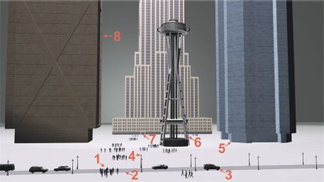
FIGURE 2.1 The polyspatial nature of the model can support multiple representations of geography in one simulation. An urban scene can hold representations of (1) social geography within a group of friends; (2) transport geography of road links; (3) vehicular movement on a network space; (4) street infrastructure as way-finding markers for agents’ behavioral geography; (5) geometry of buildings for path planning in an informatics space; (6) landmarks and meaning in cultural geography; (7) doors for entry to spaces in a time geography; (8) internal building plans within an architectural space
Second, there must be support for multiple representational geographies for agents in the model, such that their geographic abilities, appearance, and the information that they convey in simulation becomes polyspatial. Of course, this means allowing three-dimensional matrices for agents’ geography, replacing one-dimensional representations on two-dimensional planes that are commonly employed. For example, I represent individual agents as fully articulated rigs composed of vertices (joints) and (weighted) edges (bones) that may be dynamically positioned in space and time relative to constraints of realistic human skeletons (Torrens, 2012). This allows agents to articulate their movement through space and time using stride, poise, gait, and body language, rather than simply updating a one-dimensional vector. Agents can also pivot, turn, sidestep, slide, and fall over if necessary. With one rig representation, we can also wrap agents with enveloping meshes to give them corporeal form, and even clothing (Figure 2.2). For collision detection, we may reduce agents to a simple capsule or cylinder to ease calculations of overlap. For animation and communicating results to users, we can texture agents so that they look realistic relative to real-world scenes.
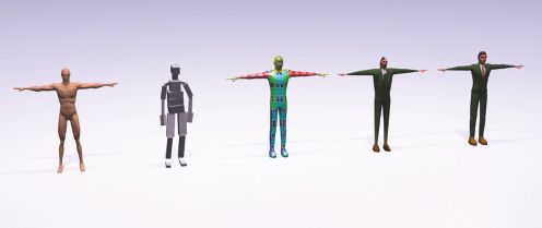
FIGURE 2.2 Multi-representational geographies for agents’ bodies. From left to right: a non-uniform rational B-spline envelope for heightened realism relative to real-world scenarios; a block model for collision detection; a three-dimensional texture map; a low-polygon texture-mapped geometrical skin
Third, as a consequence of polyspatiality in spatial reference and representation, agents are afforded a range of interaction schemes. This includes interactions within agents’ own cognition, between agents and other agents (Torrens and McDaniel, 2013), and between agents and the environment (in whatever form they consider it) (Torrens, 2014). These interactions are already common for agents as part of multi-agent systems (Ferber, 1999). However, further interactions are required between and within environmental components of the model to factor in these dynamics. The environment, in this context, can take on a variety of forms. And dynamics in one environment can pass via interaction into other model environments during simulation. In this way, interaction is polyspatial in its ability to translate interaction signals between agents, systems, and representations. Of most immediate relevance to the agent, agent rigs are ensembles of nodes and links that assume environmental form in considering agent dynamics, when, for example, an agent must determine how a movement in one part of their body should produce an action or reaction in another, or how that system of interactions should be influenced by the streetscape environment while walking, or by other agents’ skeletons when avoiding collisions (Torrens, 2012). Similarly, the interactions of building components during a collapse scenario may be handled using a physics model and then translated as dynamic geometries to agents’ visual systems and translated into steering interactions via movement (Torrens, 2014).
Fourth, systems (including the objects that populate them) are polyspatial in their processes. Agents – however they are considered or represented in the model – can be driven by (or subject to) a variety of process models, simultaneously in simulation. This allows a model user to better represent the real world in simulation, by building in diverse phenomena for agents to contribute to. It also expands the range of scenarios that can be explored in simulation, as agents can be parameterized and then subjected to different model processes without (necessarily) changing the parameterization (Torrens, 2009). As with interaction, processes can also be translated from one model scheme to another (Torrens et al., 2013; Zou et al., 2012). Indeed, this latter ability is crucial in representing surprising events that agents may encounter, in which agents must try to reason about the dynamics that are unfolding around them, using the model behaviors that they have on hand in their own abilities and cognition (Torrens et al., 2011). In this way agents are able to react to what is going on around them, without needing to know why or how the dynamics are taking place: they can have a shallow reaction to a deep process (or vice versa).
Fifth, the systems in which we embed and explore agents are polyspatial in their consideration of scale. We are often interested in the scaling of a system, its form at one phenomenal level relative to another, from one observational range to another, or from dynamics of an individual to that of a population (Batty and Longley, 1994). Similarly, we may be interested in how allometry holds at a given scale or persists across scales as fractal, recursive, or other forms. Indeed, the emergence of phenomena in three dimensions is largely under-explored in many geographical ABMs, although the topic is of critical significance in other geographical domains, including medicine (Coffey, 1998) and biology. Scale and scaling is critical in urban applications of ABMs, and examples are easy to consider (although tough to simulate): how the macro-state of a building relates to its micro-fragments in a collapse scenario; how the macro-kinematics of a body in motion is determined by micro-rotations and translations between bones through a joint (Figure 2.3); how the macro-observation of a crowd collective forms from and informs the microcosm of decisions that crowd members take to step in one place or another, and so on (Batty, 2005). We must also consider temporal scale and scaling in geographical ABMs, even when systems, models, or phenomena operate at varying rates of update and change, from the sub-second awareness and calculations of human movement to many fractions of a second considered in the physics of building interaction during an earthquake.
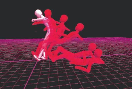
FIGURE 2.3 The model can handle scaling across all entities and objects in the system, as well as considering scaling within entities. The three-dimensional positioning and rotating of an individual joints and main corporeal system (axial skeleton for posture and center of gravity, and the appendicular skeleton for locomotion and ambulation) can be treated in isolation or in groups designed to accomplish a kinematic goal (such as protecting against a fall) relative to space and time. These sorts of dynamics would be incredibly difficult to accomplish in a two-dimensional model
Sixth, there is often some operational need to support polyspatiality in model assumptions for diverse computation, particularly when, say, ABMs need to interface with calculation, estimation, and processing schemes that are conventional to other forms of spatial simulation (and those that are non-spatial). This occurs, in particular, when the results of geographical ABMs need to be translated into numerical simulations (Kevrekidis et al., 2003), which may often be three-dimensional in nature and which handle computation using voxel-based strategies for collecting input and distributing processing. Also, components of ABM simulation may require diverse computation and calculation to realize different components of simulation, from spatial indexing and geographic information access to rendering and animation (Figure 2.4).
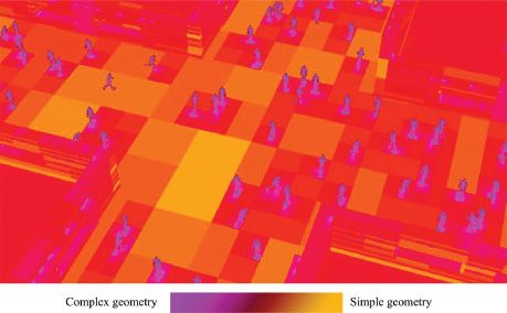
FIGURE 2.4 The three-dimensional (voxelized) view of a frame of animation for an agent-based model of an urban streetscape. The renderer bins the geometry of the scene by triangle count, devoting more in-depth computation (lighting, culling, ray-tracing, reflection, ambient occlusion) to portions with relatively high triangle counts or complex textures. As a result flat and featureless surfaces with no shadows require less computation and assume large voxels, while detailed meshes such as agent envelopes require relatively small voxels and more computing
Some examples
In the examples that follow, I will demonstrate how polyspatial agents can be usefully employed to represent geographical phenomena in three dimensions of space, proceeding beyond the existing capabilities of traditionally favored two-dimensional approaches. The first example tasks agents with handling complicated ensembles of humans in crowded settings; the second example looks at interactions between humans and a highly dynamic built environment.
Three-dimensional crowds of three-dimensional people
Many ABMs have been designed to explore the geography of individuals as mobile entities within crowd aggregates; for an excellent overview of the field, see Pelechano et al. (2008). Indeed, the emergence of crowd-level phenomena from the individual interactions of mobile agent walkers is one of the often-cited exemplars of complex adaptive systems (Ball, 2003; Batty et al., 2003a; Bouvier et al., 1997; Farkas et al., 2002; Helbing et al., 2000, 2005; Helbing and Molnár, 1997; Henein and White, 2007; Hoogendoorn and Bovy, 2000; Moussaïd et al., 2011; Partridge, 1982; Raafat et al., 2009; Stanley, 2000; Strogatz, 2004; Zhang, 2009). Crowd simulations also have significant practical potential, as they may be used to explore dynamics of crowd problems such as congestion, stampedes, and crushes (Harding et al., 2010), in which crowds must assemble and move in limited space. If one considers the experience of being part of a tightly packed crowd, it is perhaps apparent that the complications associated with the phenomenon rely quite significantly on three dimensions of space. Crowd ensembles in these instances are often crowded, that is, people impinge upon each other’s personal space (Gérin-Lajoie et al., 2008; Habicht and Braaksma, 1984; Sobel and Lillith, 1975), they interact physically (Ciolek, 1978; Daamen and Hoogendoorn, 2003; Goffmann, 1971), and they must negotiate significant obstacles in their vision and degrees of freedom in movement (Batty, 1997b; Boulic et al., 1994; Foltête and Piombini, 2007). In many cases, the available volume of space around an individual crowd participant becomes so constrained that they must succumb to reactive behavior in close quarters – they become locked into small perturbations in the space–time dynamics around them, even when their desires for movement suggest alternative behavior (Figure 2.5).
Generally, many geographical ABMs of crowd congestion are modeled using one-dimensional point masses on two-dimensional planes (Helbing and Molnár, 1995), and they completely miss the third dimension. Variants that use extruded three-dimensional cylinders (van den Berg et al., 2008) or playback animation of agent avatar representations for visualization purposes (Crooks et al., 2009) still often retain this 1D/2D behavioral representation at their cores. Abstracting from the third dimension is useful and convenient, largely because it allows vectors to be mapped to point masses and for physical forces to be calculated between those masses as if they were particles (Henderson, 1971; Treuille et al., 2006). Convenience in this context does not yield realism, and significant details are missed in the abstraction which creates a requirement for results from such models to often be explained in aggregate form (level of service, flow rates, traversal potential, etc.). Furthermore, 1D/2D models often produce problematic artifacts such as spongy compression and expansion in crowd formations (realistically, tightly packed crowds rarely move backwards unless ordered to do so with coordinated help from outside actors), and unrealistic spinning/rotation of point masses (which gives agents unrealistic abilities to see in 360 degrees of vision) (Torrens et al., 2012).
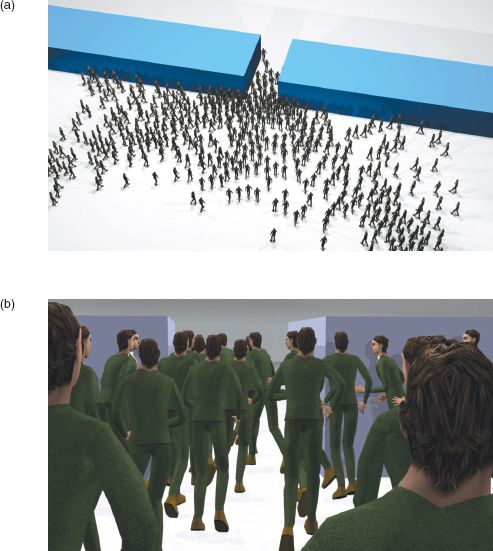
FIGURE 2.5 A frame from the crowd model from (a) a holistic view and (b) up close within the crowd, showing the significance of three dimensions in constraining the degrees of freedom that walkers have in movement and acquisition of geographic information from their surroundings
To address these limitations, I extended the representation of synthetic human agents in the model, to give them three-dimensional skeletons (Figure 2.6) and to represent the dimensionality of their skeletons in the simulation. The added dimensionality has consequences for other components of the simulation. Collision detection and resolution must be performed in three dimensions (which is achieved by adding collision spheres to the rig), and locomotion can now consider ambulation of the agents’ bodies (which I enabled through inverse and forward kinematics subject to motion-captured constraints). Similarly, I allowed agents to view their surroundings in three dimensions, using frustums in lieu of ray-casting (Figure 2.7). These representations can interact with traditional 1D/2D schemes if needed; for example, vectors for movement can be mapped to agents’ center of gravity and projected to the plane.
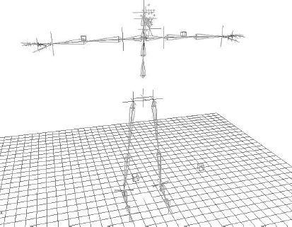
FIGURE 2.6 To allow agent rigs to physically interact in three dimensions during simulation, we added collision spheres (yellow) to key nodes and extremities (b) atop the basic skeletal rig configuration (a)
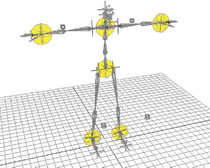
FIGURE 2.7 The three-dimensional characterization of the agents and ambient built environment extends into their vision so that they can collect three dimensions of spatial information as they act, react, and interact in the simulation
The net result is a model with significant added detail, in its dimensionality, and also in its process models. For similar scenarios, such as the well-known challenge of crowd egress through a single-exit room, the three-dimensional model yields substantively different results than standard approaches. Traditional artifacts of simulation disappear and different patterns emerge, such as irregular assembly patterns around congested exits (Figure 2.8). Moreover, we can explore both collective and individual patterns of movement and interaction in the model as ensemble behaviors and outcomes are appropriately sourced in individual behavior and geographic information (Figure 2.8).
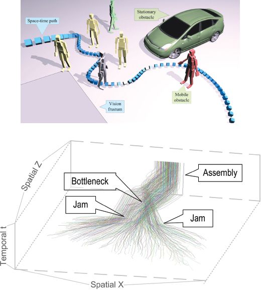
FIGURE 2.8 Space–time paths for individual agents in the room-egress scenario. Collective patterns of jamming, bottleneck congestion, and assembly are evident in the informational signatures of agents’ movement, and the contribution of each and every action of the agents to those patterns can be explored in individual or collective form
Dynamic three-dimensional built substrates for agent behavior
The scenario discussed above considers the dynamics of individuals and crowds relative to a static built environment. Assumptions of built rigidity and stability are usually realistic, as most urban infrastructures do not change on the spatial and temporal scales of agent movement. There are, however, exceptional conditions under which the built environment does move, as during earthquakes, for example (Anagnostopoulos, 1988; Villaverde, 2007). In these instances, we must consider the three dimensions of agents and crowds, but also the space–time dynamics of building fracture and collapse. This is not straightforward, because the processes that generate building dynamics in earthquake scenarios are quite different than those that drive deliberative human movement and locomotion. A coupling between two model systems is thus required, and we need to allow for the exchange of information, objects, and processes between these systems if we are to generate realistic geographical dynamics at the built–human interface.
To achieve this, I extend the idea of polyspatiality to the built environment representations and processes in the model, by allowing for physical processes of fracture, friction, and Newtonian force between the geometry and masses of the built infrastructure. By assuming the passage of energy from seismic activity through modeled objects in simulation, we can determine appropriate fracture patterns and then model the formation of new objects, as well as forces between objects as they collide in space and time. This is shown in Figure 2.9 for a set of simple geometric solids, and for a synthetic representation of an urban area built from LiDAR data in Figure 2.10 (Torrens, 2014). The dynamics from the physical simulation of building collapse pass directly into the crowd simulation as they should – as geometries for human agents to see, avoid, and plan around. In addition, as the built environment changes, so too do the features of the agents’ mental map of the city: existing goals may disappear, known paths may vanish, and lines of sight may become obscured. Because the model is built in three dimensions, agents may walk over and pass under debris as they move through the simulated scenarios.
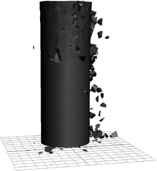
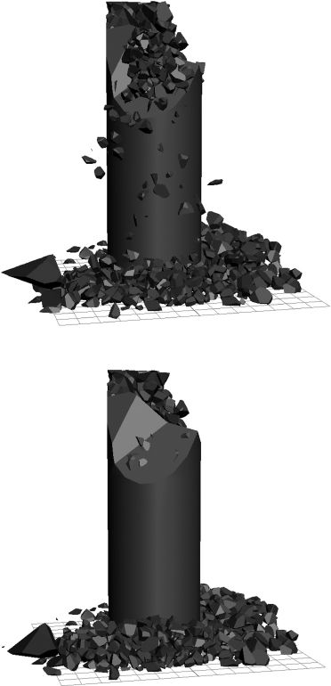
FIGURE 2.9 Dynamic, physical interactions among forming objects as a solid geometry fractures and collapses
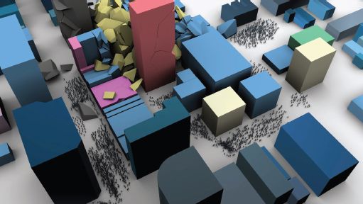
FIGURE 2.10 A frame from the earthquake evacuation model, showing agents reacting both to each other as they form congested crowds, and to the dynamic changes in the built environment following building collapse and shifts in the urban fabric around them
Conclusions
In this chapter, I have argued in favor of increased dimensionality in considering, representing, running, and examining geographical agent-based models. Motivated primarily by a quest for increased detail and realism in geographical ABMs, I have proposed that more useful models and simulations can be built and applied with added dimensionality, owing in large part to the expanded range of questions that can be explored in three dimensions but are simply not accessible in two-dimensional ABMs. In support of my point, I introduced two simulation scenarios: one involving tightly packed three-dimensional crowds and another that expands on this scenario by including dynamic collapse scenarios in the built infrastructure of a simulated city. More intricate details of how these models work, and the innovation that underpins them, are provided in Torrens (2012, 2014).
It is worth noting that as geocomputational models using agent-based representations of people and things that we experience and sense in the real world begin to add dimensionality and detail, and as our data resources to ground such models in reality expand and refine, we will also begin to move away from traditional ideas of models themselves. In classical spatial simulation, models are usually considered as scaled versions of complicated realities. They have, in the past, been built as pedagogical tools or as estimators, usually with abstraction or coarse appreciation as an aim. In recent years (and perhaps steadily throughout the evolution of such models), an alternative narrative regarding the use and potential of spatial models has developed, one in which the model presents as a synthetic reality, a computational laboratory for playing with ideas, plans, and fancies. While scaled models may always have significant value in the scientific process, it is likely that geographical ABMs will enjoy increasing use as engines for geography in developing virtual worlds and augmented realities in the future.
FURTHER READING
Stan Openshaw’s early papers (e.g. Openshaw et al., 1987) set the stage for most of what we now call geographical ABMs, by introducing advanced notions of computation and computability, and by proving that geography is everywhere in the computational realm. Paul Longley’s edited book on geocomputation was pivotal in organizing the field around a common research agenda and in introducing its defining concepts (Longley et al., 1998). Readers of this particular chapter may be interested in exploring geosimulation models in Benenson and Torrens (2004), which presents a very detailed overview of the last 50 years or so of geocomputational simulation methods and applications. Andrew Crooks and colleagues have also published a more recent book on geographical agents with contributions from a range of authors in the field (Heppenstall et al., 2012). Michael Batty’s (1997a) paper on the computable city is a must-read, as in many ways it predicted the now rapidly appearing fusion of models and data that is coalescing around the notion of a new science of cities, which is largely mediated by geocomputation. His recent book on that very topic is also a useful resource (Batty, 2013). Jean Baudrillard saw the clash of models and reality coming a long time ago, and this is discussed philosophically in Simulacra and Simulation (Baudrillard, 1994). Science is always inspired and contextualized by science fiction, and readers may wish to refer to Neal Stephenson’s (1993) book on virtual worlds and avatars, Snow Crash, for particularly relevant insight. My opinion is that it is all about geography!
All materials on the site are licensed Creative Commons Attribution-Sharealike 3.0 Unported CC BY-SA 3.0 & GNU Free Documentation License (GFDL)
If you are the copyright holder of any material contained on our site and intend to remove it, please contact our site administrator for approval.
© 2016-2026 All site design rights belong to S.Y.A.