Geocomputation: A Practical Primer (2015)
PART II
EXPLORING MOVEMENTS IN SPACE
4
AGENT-BASED MODELING AND GEOGRAPHICAL INFORMATION SYSTEMS
Andrew Crooks
Introduction
Modeling human behavior is not as simple as it sounds. This is because humans do not just make random decisions, but base actions upon their knowledge and abilities. Moreover, one might think that human behavior is rational, but this is not always the case: decisions can also be based on emotions (e.g. interest, happiness, anger, fear). Emotions can influence decision-making by altering an our perceptions about the environment and future evaluations (Loewenstein and Lerner, 2003).
The question therefore is how we model human behavior. Over the last decade, one of the dominant ways of modeling human behavior in its many shapes and forms has been through agent-based modeling (ABM) (see also Torrens, Chapter 2). The remainder of this chapter provides a general overview of what agents are, why there is a need for agent-based models for studying geographical problems, and how it links to how we believe societies operate through ideas of complexity theory. It sketches out how geographical information can be used to create spatially explicit agent-based models, before reviewing a range of applications where agent-based models have been developed using geographical data. The chapter concludes with an overview of challenges modelers face when using agent-based models to study geographical problems, and identify future avenues of research.
What are agents?
ABM allows us to focus on individuals or groups of individuals and give them diverse knowledge and abilities (Crooks and Heppenstall, 2012). This is possible through the unique properties one can endow upon the agents (people, animals, etc.) within such models (Heppenstall et al., 2012; O’Sullivan and Perry, 2013). The key difference between ABM and other forms of modeling is the ability to focus on the individual and their behaviors. These properties include:
• Autonomy: We can model individual autonomous units that are not centrally governed. Through this property agents are able to process and exchange information with other agents in order to make independent decisions
• Heterogeneity. Through using autonomous agents the notion of the average individual is redundant. Each agent can have their own properties and it is these unique properties of individuals that cause more aggregate phenomena to develop.
• Activeness. As agents are autonomous individuals with a range of heterogeneous properties, they can exert active independent influence within a simulation. There are several ways agents can do this: they can be proactive (goal-directed), as when trying to solve a specific problem; or they can be reactive, in the sense that they can be designed to perceive their surroundings and given prior knowledge based on experiences (e.g. learning) or observation and take actions accordingly.
The primary strength of ABM is as a testing ground for a variety of theoretical assumptions and concepts about human behavior (Stanilov, 2012) within the safe environment of a computer simulation. For example, we know humans process sensory information about the environment, their own current state, and their remembered history to decide what actions to take, all of which can be incorporated with agents (Kennedy, 2012). Through the ability to model heterogeneity within agent-based models we can capture the uniqueness of what makes us human, in the sense that all humans have diverse personality traits (e.g. emotion, risk avoidance) irrational behavior, and complex psychology (Bonabeau, 2002). We also know that human behavior is influenced by others (e.g. Friedkin and Johnsen, 1999), which can introduce positive and negative feedbacks into the system. Through such processes, people form groups, and the results of aggregate behavior can be greater than the sum of the individuals within the group. Such properties again can be captured through the agents heterogeneity and active status.
But what drives humans? What motivates us to take certain actions? By agents being active we can test ideas and theories on what motivates people, and explore why do they do certain things. Perhaps the most cited concept in this regard is Maslow’s (1943) ‘hierarchy of basic needs’; Maslow discussed how humans order their needs and provided an overview of potentially competing priorities when trying to represent human behavior within an agent-based model. Kennedy (2012) lists three main approaches to capturing such cognitive processes, the first being a mathematical approach such as the use of ad hoc direct and custom coding of behaviors within the simulation, as when using random number generators to select a predefined possible choice (e.g. to buy or sell; Gode and Sunder, 1993). However, as noted above, people are not always random, which has led researchers to develop other methods such as directly incorporating threshold-based rules. For example, when an environment parameter passes a certain threshold, a specific agent behavior will result (e.g. move to a new location when the neighborhood composition reaches a certain percentage; Crooks, 2010). One could argue that such modeling approaches are appropriate when behavior can be well specified.
The second approach to modeling human behavior is through the use of conceptual cognitive frameworks. Within such models, instead of using thresholds, more abstract conceptual frameworks are used, such as beliefs, desires, and intentions (BDI; Rao and Georgeff, 1991), or physical, emotional, cognitive, and social factors (PECS; Schmidt, 2002). Both the BDI and PECS frameworks have been successively applied to modeling crime patterns (see Brantingham et al., 2005; Pint et al., 2010). These conceptual cognitive frameworks are basically decision tree hierarchies with respect to guiding human behavior within agent-based models, and offer a bridge between mathematical representations of behavior and those research-quality cognitive architectures tools that we will turn to next. While the approaches above have been developed with respect to ABM, research-quality cognitive architectures focus on abstract or theoretical cognition (Kennedy, 2012), with two of the most widely used architectures being Soar (Laird, 2012) and ACT-R (Anderson and Lebiere, 1998); however, such architectures tend to focus more with artificial intelligence and matching human decision-making over very short periods of time (seconds to minutes) on a small number of agents.
Why agent-based modeling?
The growth of ABM coincides with how our views and thinking about how social systems such as cities are being changed by utilizing ideas from complexity science (see Manson et al., 2012). Rather than adopting a reductionist view of systems, whereby the modeler makes the assumption that cities operate from the top down and results are filtered to the individual components of the system (see Torrens, 2004), people are now adopting a reassembly approach to the system, in the sense of building the system from the bottom up (O’Sullivan, 2004). This change follows the realization that planning and public policy do not always work in a top-down manner; aggregate conditions develop from the bottom up, and from the interaction of a large number of elements at a local scale. Thus there is a move toward individualistic, bottom-up explanations of geographical form and behavior which link to what we know about complex systems (Batty, 2005).
The key characteristics of complexity – such as self-organization, emergence, non-linearity, feedback and path dependence – can all be captured within agent-based models. By their very nature, agent-based models can capture emergent phenomena which are characterized by stable macroscopic patterns arising from local interaction of individual entities (Epstein and Axtell, 1996). A small number of rules or laws, applied at a local level and among many entities, are capable of generating complex global phenomena: collective behaviors, extensive spatial patterns, hierarchies, and so on, which are manifested in such a way that the actions of the parts do not simply sum to the activity of the whole. Thus, emergent phenomena can exhibit properties that are decoupled from (i.e. logically independent of) the properties of the system’s parts. For example, a traffic jam often forms in the opposing lane to a traffic accident, a consequence of ‘rubber-necking’ (Masinick and Teng, 2004).
To give a simple example of how ABM can be used to study such an issue, take Figure 4.1, where each car is an agent and is given two very simple rules of and second, if there is no car in front, the car speeds up. These two simple rules applied to many agents can demonstrate how traffic jams can form without any serious incident. Moreover, through the modeling of individuals, we can see that there is great variation between individual car speeds that would be lost if we only looked at the aggregate (average) speed of traffic (such behaviors are explored in more detail later). However, if you are wondering if such simple rules can explain the emergence of traffic jams, see Sugiyama et al. (2008).
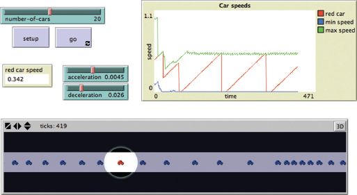
FIGURE 4.1 Simple traffic model where each car is an agent. From top left clockwise, model parameters, a chart of car speeds and the spatial agent environment (source: Wilensky, 1997, 1999)
Studying the behavior of collections of entities focuses attention on relationships between entities (O’Sullivan, 2004) because before change is noticed at the aggregate level, it has already taken place at the micro level. Complexity theory has brought awareness of the subtle, diverse, and interconnected facets common to many phenomena, and continues to contribute many powerful concepts, modeling approaches and techniques especially in relation to ABM. Geographical systems provide many examples of self-organization and emergence (Heppenstall et al., 2012; Batty, 2013); for example, it is the local-scale interactive behavior (commuting, moving) of many individual objects (vehicles, people) from which structured and ordered patterns emerge in the aggregate, such as peak-hour traffic congestion (Nagel et al., 1997) and the agglomeration of firms (Krugman, 1996b).
Why link GIS and agent-based models?
As noted above ABM has relevance to many geographical problems and there is growing interest in the integration of GIS and ABM through coupling and embedding (see Crooks and Castle, 2012, for a review). For agent-based modelers, this integration provides the ability to have agents that are related to actual geographic locations. This is of crucial importance with regard to modeling geographical systems, as everything within a city, region or country is connected to a place. Furthermore, it allows modelers to think about how objects or agents and their aggregations interact and change in space and time (Batty, 2005). For GIS users, it provides the ability to model the emergence of phenomena through individual interactions of features within a GIS over time and space. Moreover, some would consider this linkage highly appealing in the sense that while GIS provides us with the ability to monitor the world, it provides no mechanism to discover new decision-making frameworks such as why people have moved to a new area (Robinson et al., 2007).
The simplest way to visualize the integration of GIS and ABM is by taking the view most GISs do of the world, as shown in Figure 4.2. The world is represented as a series of layers (such as the physical environment, the urban environment) and objects of different types (such as cars or people, which can then be used as the basis for our agents). These layers form the artificial world for our agents to inhabit; they can act as boundaries for our simulations, or fixed layers such as roads provide a means for agents to move from A to B or houses provide them with a place to live. To further illustrate this notion, in Figure 4.3 we show a modified SLEUTH1 model (Clarke et al., 1997). The model predicts the extent of urban growth, for example, from blue for the current urban extent, to red for the possible future urban extent after the model has been initialized with the input data and applying specific growth rules controlled by specific growth coefficients (see Clarke et al., 1997, for more details). Aggregate spatial data also allow for model validation: for example, are the land-use patterns we see emerging from a model of urban growth matching that of reality? If they do, it provides us with an independent test of the micro-level processes encoded within the model. Taking the example above, the growth coefficients can be calibrated and validated by comparing simulated land-use change with historical geographical information on the area, and if the model matches reality we can be more confident with future growth strategies.
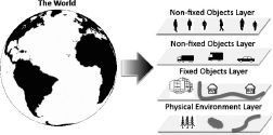
FIGURE 4.2 Representing the world as a series of layers of fixed and non-fixed objects (adapted from Benenson and Torrens, 2004)
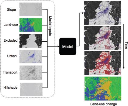
FIGURE 4.3 A basic SLEUTH-type model based on growth rules and coefficients as outlined in Clarke et al. (1997) driving the rates of land-use change in Santa Fe, New Mexico at 30 m2 resolution
However, it is not just raster data that can be used as the basis for the artificial world, but also vector data. For example, translating vector data into agents and their environment is shown in Figure 4.4. Here the model comprises two vector layers: the urban environment is represented as a series of polygons created directly from the shapefile; and agents are represented as points. It is the information held within fields of the environment layer (Figure 4.4(a)) that is used to create the point agents (Figure 4.4(b)), but also the layer extent defines the boundary of the world (see Crooks, 2010, for further details). The agent-based model uses the data to initialize the model. Note that the underlying color of the polygon can be used to represent the predominant social group in the area (accomplished by counting the number of agents (points) of different types within each polygon). Once the agents have been created they can be given simple rules; for example, in Figure 4.5 we show a model inspired by Schelling’s (1971) model of segregation, where each agent has a preference of living in a neighborhoods where 50% of their neighbors are like themselves. Agents then calculate through a buffer operation their neighborhood makeup, and if their preferences are not met (i.e. 50% of their neighbors are not like themselves) they move to a new location where their preferences are met. Through such rules we can explore how the actions of many individual agents result in, say, the emergence of segregation at different levels of aggregation, as shown in Figure 4.6.
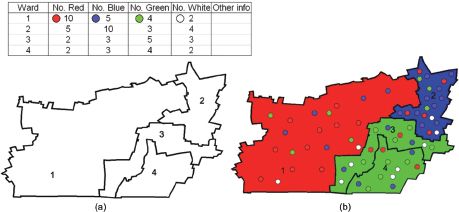
FIGURE 4.4 Populating a model with agents: (a) the environment layer and corresponding attribute fields; (b) reading in the data and creating the environment and the agents based on the attributes of the fields
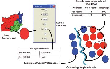
FIGURE 4.5 Basic segregation model structure
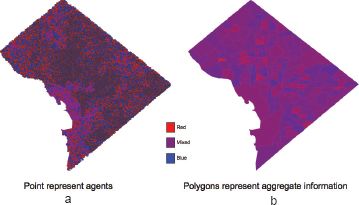
FIGURE 4.6 Segregation within areas and across boundaries: (a) the entire area with individual agents represented; (b) the aggregate information, where each Census block is shaded depending on the most dominate social group
Example applications
Agent-based models have been created to study a diverse range of geographical phenomena (see Heppenstall et al., 2012),2 and this section provides only a brief review of such applications. The intention is to show how one can use agent-based models to study a diverse range of phenomena at different spatial and temporal scales such as those shown in Figure 4.7. These range in temporal scale from the split-second decision-making involving local movements such as people walking, traffic modeling over minutes and hours, residential movement (e.g. Crooks, 2007; Malik et al., 2013) and urban growth over months and years, through to the migration of people over decades (e.g. Gulden et al., 2011; Pumain, 2012). However, it needs to be noted that agent-based models can be used to study a wide variety of fields, such as ecology (e.g. Grimm and Railsback, 2005), biology (e.g. Kreft et al., 1998), and geomorphology (e.g. Reaney, 2008), to name but a few. That being said, we now turn our attention to models that involve humans and space.
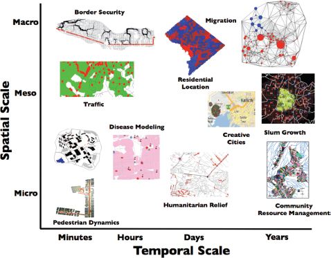
FIGURE 4.7 A sample of application domains for spatial agent-based models
As noted above, agent-based simulations serve as artificial laboratories where we can test ideas and hypotheses about phenomena that are not easy to explore in the ‘real world’. One example of this is pedestrian modeling of evacuation or movement in general. For example, without actually setting a building on fire we cannot easily identify people’s reactions to such an event. ABM, as with simulations in general, can allow for such experiments. Rather than setting a building on fire, we can re-create the building within an artificial world, populate it with artificial people, start a fire and watch what happens. Such simulations allow the modeler to identify potential problems such as bottlenecks and allow for the testing of numerous scenarios such as the way various room configurations can impact on evacuation time. By building such models we can focus on mitigation and preparedness rather than response and recovery in emergency incident management.
Building the spatial environment of such models is relatively straightforward, as shown in Figure 4.8, for example. From an architect’s CAD file of a building we can georeference the building to its actual ‘real-world’ location. We then take the building and rasterize the space so that each cell represents, say, 50 cm2, which approximates the anthropomorphic dimensions of an individual (Pheasant and Haslegrave, 2006). This regular lattice structure is used for our artificial world in a similar way to that of other pedestrian models (e.g. Batty et al., 2003b); however, a continuous (i.e. vector) space representation could also be used if so desired (see Castle, 2007, for a discussion of the role of space within pedestrian models). Once we have the spatial layout of the building, we can then populate the building with agents that have simple rules; for example, once the alarm is activated, agents follow emergency signage (or move to the nearest exit). This process is shown in Figure 4.8(c) and (d). The simulation demonstrates how bottlenecks form at exits and how this causes agents to cluster around such obstacles.3
It is not just evacuation models that can benefit from utilizing agent-based models. Such models have been developed to explore a wide range of phenomena where the movement of people plays a critical role (see Torrens, 2012), for example, event safety (e.g. Batty et al., 2003b), and understanding how people move around town centers (e.g. Haklay et al., 2001) or theme parks (e.g. S.-F. Cheng et al., 2013). Geographically explicit pedestrian models have also been developed to explore how people find out and search for food in times of crisis (e.g. Crooks and Wise, 2013). and to explore the spread of diseases within refugee camps (e.g. Crooks and Hailegiorgis, 2013).
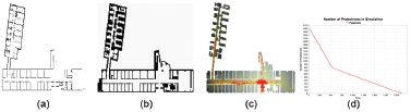
FIGURE 4.8 Simple pedestrian model: (a) CAD floor plans of a building are converted into (b) a raster layer and are used as the environment for the agent-based model. (c) shows the simulation running with agents (red) who are exiting the building and leaving behind walking traces (yellow). (d) shows a time series plot of agents evacuating from the building
Moving from the small-scale interactions of pedestrians, agent-based models have also been developed to explore how people navigate through space, and the results of these behaviors in aggregate. Such models have been developed to understand and potentially reduce traffic congestion or pollution, for example (Helbing and Balietti, 2011). ABM is ideal for studying the effects of traffic, as each vehicle and potentially each entity of the simulation (e.g. traffic lights) can be represented as individual objects or ‘agents’ which make independent decisions about their actions. Behavior can be incorporated into such models; for example, how many individuals can cause traffic jams (Nagel and Schreckenberg, 1992), how different road-pricing scenarios influence usage (e.g. Takama and Preston, 2008), how traffic conditions can be simulated over entire countries (e.g. Raney et al., 2003), and how people find a place to park (e.g. Benenson et al., 2008).
Geographical information plays a critical rule in such models. For example, in the model presented in Figure 4.9, we explore commuters who are working within the Tyson’s Corner area of Virginia on the border of Washington, DC. We take road and travel-to-work data from the US Census as the basis for our spatial agent-based model. The road data act as a basis for our agents to move from their homes to Tyson’s Corner, and the Census data provides us with the number of agents who travel to the area on a daily basis. The agents attempt to find the shortest path from their home to their destination, with preferential attachment to highways and freeways over smaller country roads. By running the model, cars start at homes and travel towards Tyson’s Corner, and as more cars join certain sections of roads, traffic jams start to form (as speed is a function of the number of cars on a specific section of road). For example, in Figure 4.9(b), individual cars can be distinguished when they are not clustered, but when traffic density increases, larger clusters develop. Such a model could easily be extended to incorporating a range of route choice behavior (e.g. Manley et al., 2014).
Researchers have also combined traffic models of cars with those of pedestrians. For example, Banos et al. (2005) explored the interaction of pedestrians and vehicles within the urban street network, with the aim of understanding how one can reduce the number of casualties from vehicles. In another model, Łatek et al. (2012) explored how an agent-based model could be used to understand dynamics along the US–Mexico border – specifically, how border security infrastructure (e.g. integrated fixed towers) can impact on the prevalence of smuggling (e.g. of drugs or people), by modeling both pedestrians and vehicles. Figure 4.10(a) outlines the data layers needed to explore this question.
Within the model, land cover and terrain relief are used to calculate viewsheds for the placement of security infrastructure via line-of-sight analysis. As the model is also interested in routing across the border and for border patrol agents, roads and terrain roughness are also needed, as this enhances or impedes movement. However, as the model incorporates the movement of smugglers, one also needs to incorporate geographical information that impacts on behavioral routing decisions. This includes population density, in the sense that smugglers initially do not want to be seen and therefore avoid highly populated areas, along with land ownership that elicits different access constraints. Once such information is obtained, we can then simulate how smugglers and border protection agents might interact on this terrain, as is shown in Figure 4.10(b). We can also validate such movement patterns based on real-life drug seizures whose locations are made publically available.
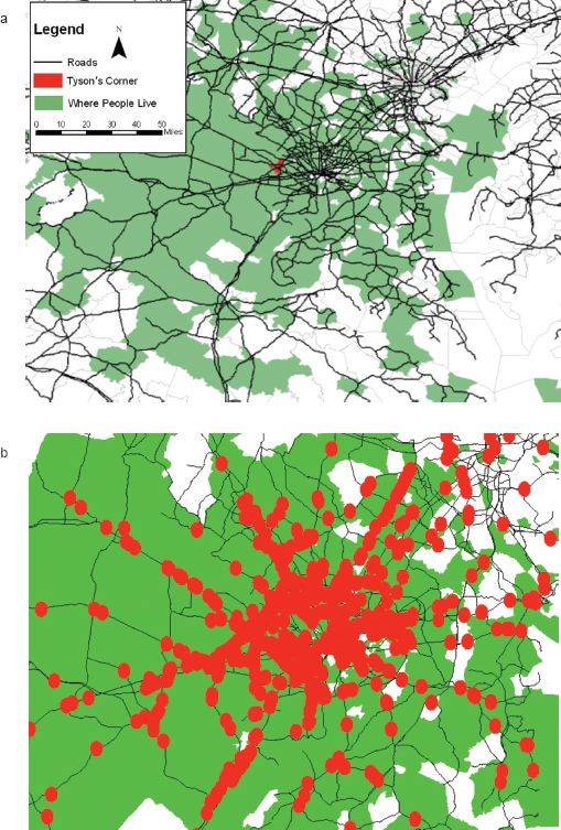
FIGURE 4.9 Using agent-based models to explore rush-hour congestion: (a) road and Census data used for model inputs; (b) zoomed-in section of (a) with agents (red circles) moving towards Tyson’s Corner and causing traffic jams
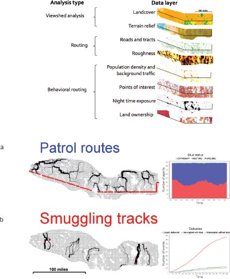
FIGURE 4.10 Modeling border security along the Arizona–Sonora borderland: (a) data layers and analysis type for the simulation; (b) visualization of the model, showing both patrol routes and smuggling tracks
Cities have continued to grow over the last 200 years and there is little sign of such growth slowing down. Physically, they can grow in two different ways: expansion and compaction. The process of expansion leads to more space being occupied (e.g. sprawl); compaction leads to the same amount of space being occupied by more people, resulting in increased population density. Not only do cities grow physically, but they also change their resourcing demands; for example, they may require more water, building materials, food, goods, and services from the surrounding region, which results in population, economic activities and technology diffusion. The motivations for modeling urban growth processes should be obvious. If we can understand and estimate such growth, we can not only raise awareness of the consequences of urban growth, but also test out policy ideas (e.g. restricting growth on specific land-use types or promoting higher-density development) to see how these policies might impact future land-use patterns.
While urban modeling has a long tradition (e.g. Batty, 1976), recently researchers have started to explore such issues through agent-based models due to specific limitations of past modeling endeavors (see Benenson and Torrens, 2004). For example, Torrens (2006) combined GIS data and ABM to explore urban sprawl in Michigan, while Xie et al. (2007) explored urban growth in China, specifically focusing on the pressure on land from developers. Others have explored the evolution of land markets at the urban–rural fringe. For example, Magliocca (2012) and Wise and Crooks (2012) have explored how heterogeneous agents representing farmers, developers, and buyers could influence the spatial pattern of residential development through interactions in the land market. The results from such models are in accord with the classical urban theory (e.g. Alonso, 1964), in the sense that as the distance from the central business district increases, land prices and housing density decrease, a pattern that is also empirically observed in many US cities. By building on such models, one can explore how various planning scenarios such as lot-size zoning and municipal land acquisition strategies could reduce the impact of urban sprawl (e.g. Robinson and Brown, 2009).
Coinciding with urban growth is the rise of slums, especially in developing countries (Patel et al., 2014). Over 900 million people live in either slums or squatter settlements, a number that is projected to increase to approximately 2 billion by 2030 (United Nations Human Settlements Programme, 2003). Just as agent-based models have proved useful in exploring urban growth, they can also be a useful tool to study questions about how slums come into existence, how they expand, and which processes may make some slums disappear. For this reason several researchers have started to explore slum formation from the bottom up through ABM (Vincent, 2009; Augustijn-Beckers et al., 2011; Barros, 2012). Patel et al. (2012), however, notes that there is still much to be done with respect to modeling and improving our understanding of slums.
Conclusions
This chapter has presented a brief introduction to agent-based modeling and how such models can be linked to GIS (both in terms of raster and vector data). The applications have demonstrated how through such a linkage a wide variety of problems can be analyzed at various spatial and temporal scales. This generative (or bottom-up) approach allows us to explore how a small number of rules or laws, applied at a local level and among many entities, are capable of generating complex global phenomena at different spatial resolutions. These collective behaviors and extensive spatial patterns are manifested in such a way that the actions of the parts do not simply sum to the activity of the whole. They provide us with a new way of thinking about problems, taking ideas and insights from complexity science.
However, in conclusion, while there is great potential for ABM, there are several additional challenges that ABM faces, ranging across the spectrum of theory to practice, hypothesis to application (see Crooks et al., 2008). Validation schemes are a classic example of this. One reason why validation poses such a challenge is the degree to which the true micro-geography of any geographical system (e.g. a city) is still largely unknown in many situations. Nevertheless, this style of modeling provides a tool for testing the impact of changes in, say, room configurations, land-use type or the transportation networks in dense metropolitan areas via a simulation approach. This approach is less focused on predicting the future accurately, than on understanding and exploring the system from the bottom up.
FURTHER READING
Readers wishing to know more about ABM and GIS might be interested in the following works. For an introduction to ABM and complexity more generally, Miller’s and Page’s (2007) book Complex Adaptive Systems provides a good overview of why one might to use ABM along with considerations about how to model more generally. Gimblett’s (2002) edited book provides one of the first introductions to ABM and GIS, especially how the integration of the two can be used to study social and ecological processes, and to this day provides the foundations to many agent-based models. A more recent comprehensive edited volume of ABM applications applied at various spatial and temporal scales can be found in Heppenstall’s et al. (2012) edited volume Agent-Based Models of Geographical Systems. A detailed review of agent-based models, how they have evolved with respect to GIS and their relationship to other modeling approaches can be found in Benenson and Torrens (2004), while those interested in cities might like to read Batty’s (2005) Cities and Complexity.
1The acronym stands for the raster input datasets needed to run the model: Slope, Land-use (e.g. urban and non-urban), Exclusion (where one cannot build), Urban extent, Transportation (road network) and Hillside.
2A number of ABM toolkits have been developed to allow scientists to focus more on modeling rather than on things such as visualization of model outcomes and charting model progress. Interested readers are advised to see Crooks and Castle (2012) for a discussion on the benefits of ABM platforms which allow for GIS integration.
3Interested readers can see an animation of this model and download the source code and data along with other spatially explicit models from http://www.cs.gmu.edu/~eclab/projects/mason/extensions/geomason/.
All materials on the site are licensed Creative Commons Attribution-Sharealike 3.0 Unported CC BY-SA 3.0 & GNU Free Documentation License (GFDL)
If you are the copyright holder of any material contained on our site and intend to remove it, please contact our site administrator for approval.
© 2016-2026 All site design rights belong to S.Y.A.