Geocomputation: A Practical Primer (2015)
PART II
EXPLORING MOVEMENTS IN SPACE
5
MICROSIMULATION MODELLING FOR SOCIAL SCIENTISTS
Kirk Harland and Mark Birkin
Introduction
Microsimulation modelling has increased in popularity across a variety of disciplines over the last 60 years. The approach has become particularly prevalent in policy analysis with an emphasis on demographic and geographical implications of policy decisions. The work presented here will introduce the different ‘flavours’ of microsimulation models, including static, dynamic and spatial. Furthermore, the interface with another emergent modelling technique, agent-based modelling (ABM) (see Crooks, Chapter 4), will be discussed, followed by some examples of recent microsimulation applications. A more technical discussion will be the focus of the final section, which will suggest an architecture for a microsimulation model framework, with the trade-off between structure and efficiency considered.
What is microsimulation?
Ballas et al. (2006: 66) define microsimulation as
a methodology that is concerned with the creation of large-scale simulated population microdata sets for the analysis of policy impacts at the micro level. In particular, microsimulation methods aim to examine changes in the life of individuals within households and to analyse the impact of government policy changes for each simulated individual and each household.
Microsimulation models can be categorised into static or dynamic and whether they are spatially explicit. A static microsimulation model generates a population at a snapshot in time. A dynamic microsimulation model produces a population that is subsequently moved through time and optionally space. A microsimulation model becomes spatially explicit when population characteristics are simulated to represent realistic social heterogeneity across geographical areas.
Static microsimulation
Static microsimulation models generate a synthetic population from aggregate data, with the resulting population being immobile in both space and time. Population generation is normally a process of sampling or ‘cloning’ candidate individuals from a sample survey to create a population consistent with a series of aggregate constraint values. Where a survey population is not available for sampling, a population can be generated using the conditional probability distributions derived from the aggregate data, as demonstrated by Birkin and Clarke (1988, 1989). There are a variety of approaches for producing synthetic populations from aggregate data sources that fall into three broad categories: deterministic, statistical estimation and combinatorial optimisation. A detailed discussion of the different population generation approaches is beyond the scope of this chapter; further information on a selection of techniques can be found in Harland et al. (2012).
Dynamic microsimulation
Dynamic microsimulation models forecast past trends into the future to estimate changes in a micro-unit population (Ballas et al., 2006). As the population is moved forward through time, the likelihood of events occurring based on the characteristics of the micro-unit is assessed against probabilities derived from available data. As identified by Orcutt (1957), micro-units of the same ‘type’ have the same characteristics, but outputs for identical units need not be the same. For example, two synthetic individuals in a population aged 65, married and retired, may both have identical characteristics and the same probability (say, 0.4) of a death event occurring. However, if individual 1 has a random draw (random number generated) of 0.7 the mortality event does not occur, whereas individual 2 may have a random draw of 0.3 that results in a mortality event occurring. This demonstrates that even though many synthetic individuals can share identical input characteristics the output is dependent on the random draw and probability distribution of an event occurring, reflecting the uncertainties and decision-making processes observed in real life. Orcutt (1957) reflected that despite the variation observed, in reality a significant proportion has a relatively regular set of outputs dependent on the input characteristics of the micro-unit. This is one of the central considerations used to derive statistical risk models for managing risk exposure during the issue of personal loan and mortgages by large financial institutions and it is also, as Orcutt (1957: 118) notes, ‘because of this that insurance companies do so well’.
Probabilistic approaches may be suitable in situations where a known probability distribution for an event occurring can be derived, such as the use of life tables for mortality events. However, in some circumstances an output can be considered as a direct result of an input. Ageing may be considered this type of characteristic: an individual gets one year older, not two or three, on a particular date and only on that date. There may also be second-order implications of an event occurring. For example, if individual 1 is married to individual 2 and individual 1 has a mortality event, then a direct impact of this is that the marriage status of individual 2 will change from married to widowed.
Transitions and events
Dynamic microsimulation models can generally be categorised into either transition-based or event-based models. The difference between the two approaches centres around the way time is handled. Each approach is described briefly below.
Time-steps are the temporal currency of transition-based dynamic microsimulation models. At each time-step, events are evaluated based on the input characteristics of each micro-unit to ascertain which events take place and what the outcomes of those events are. A time-step is a discrete unit of time, normally a week, a month or a year, but any discrete measure of time can theoretically be used. Orcutt (1957) recommends relatively short periods such as a week or a month; however, the time-step of the model should be considered in the context of the intended use and the data available to derive the required event probability distributions. A model run ends when the last specified time-step is completed.
Time is treated as continuous in an event-based model. From an initial starting point, all events considered by the model have a lapse time randomly generated. The lapse time is the time to that event occurring for a particular synthetic individual. The event with the shortest lapse time is executed first. This point then becomes the starting point, and all events that are influenced by the outcome of first event have new lapse times calculated.
When events can be considered in isolation the event-based approach does have the advantage that causality can be observed (Spielauer, 2009b). The execution of an event may adjust the probabilities of another event happening, bringing the events execution forward (or perhaps pushing it back) in time. In a transition-based model, events happen between two fixed points in time and therefore causality between two events happening in the same time-step cannot be linked. It is only when the time-steps within a transition-based model become small enough for multiple events not to happen within one time-step that causality between events becomes apparent (Galler, 1997). When this is the case the transition-based model is effectively treating time as continuous. Orcutt (1957) emphasised the fact that time-steps within the transition-based architecture he described had to be of a fine enough resolution to enable the outputs of events to be considered only within the next iteration of the model and not by events within the same iteration.
Events in reality rarely happen in isolation, and therefore the relative simplicity and elegance of the event-based model is quickly lost in complex equations to account for the interdependence of events (Galler, 1997). Galler concludes that transition-based models with small enough time-steps to preclude multiple event occurrences provide the simplest and most promising architecture for dynamic microsimulation models, echoing the recommendation of Orcutt in his original paper some 40 years earlier. However, this presents another problem: the issue of model scale against processing efficiency. Despite the increases in processing power of computers and the significant fall in the cost of digital storage, synthesising and moving a large population, such as one of a whole country, is still a significant task. As noted by Spielauer (2009b), when individual micro-units can be simulated throughout their life course in isolation, an event-based approach offers the ability to process each micro-unit’s life in parallel on distributed computing networks. This reduces processing time and also offers the efficiency that only event points in the life of the micro-unit are considered, not every time-step where on many occasions nothing may happen. Again there is a conceptual trade-off with this approach. In the social sciences microsimulation models are generally used to replicate the interrelationships between events and individuals that are either not captured or ineffectively represented by aggregate approaches. To consider the life course of each individual micro-unit in isolation undermines the interrelated nature of events and individuals. Event-based models can process individual life courses simultaneously across the population to preserve relationships between individuals; however, executing the model over a distributed computing networks becomes a very complicated task.
Spatial microsimulation
Most microsimulation models have a spatial element. However, models that are spatially explicit, examining policy or demographic change at a small geographical scale (typically consisting of several hundred households), are described as spatial microsimulation models (Ballas et al., 2006). The distinction between spatial and non-spatial models is not as well defined as the difference between static and dynamic models. As noted above, most models have a spatial element, even if this is implied. The extent to which small-area demographic detail is captured within the underlying population of a microsimulation model defines the spatial resolution of the model and whether that model is described as explicitly spatial.
The explicit preservation of relationships between survey attributes at the expense of variation in small-area characteristics, such as the approach of Kao et al. (2012), assumes spatial homogeneity over small geographical areas. This approach generates a population that is attribute-rich, reflecting the underlying survey sample well, but lacks the detailed underlying spatial variation present in reality. Spatial models preserve the geographical detail by constraining the model to multiple known aggregate relationships at a small-area level, usually extracted from population census data. The spatial detail and small-area heterogeneity are included at the expense of explicitly preserving the relationships between the attributes within the sample population. Work by Smith et al. (2009) and Birkin and Clarke (2012) suggests that tailoring a microsimulation model structure, and incorporating additional information such as a geodemographic classification between survey sample and aggregate constraints, can alleviate some of these issues, thus improving population reconstruction.
Microsimulation modelling is a tool to construct theoretical arguments, aid understanding and ultimately solve complex problems. To achieve these aims, it is crucial that the researcher select the most appropriate approach for the research question under study and those data available which can feed into models. The goal of the research should inform the spatial resolution of the model and the acceptable trade-off between spatial granularity and preservation of survey detail. It should also influence whether a dynamic microsimulation model is event-based or transition-based, or indeed whether a dynamic model is required at all. It is possible that a series of static models could provide the required insights.
Agent-based modelling and microsimulation
Agent-based modelling approaches the modelling of complex systems from the activity of constituent micro-units, agents, to explore emergent macro-patterns from the micro level. Agent-based models move individual agents, expressed as discrete objects in a digital environment, through time and optionally space. The movement or behaviour of each agent is dependent on its internal state and its interactions with other agents and the surrounding environment. These inputs are processed through a set of rules or a behavioural framework contained within the agent to provide a reaction to the input stimuli (see Crooks and Heppenstall, 2012, for a good introduction to ABM concepts).
There are some obvious similarities between dynamic microsimulation and ABM approaches within the social sciences. Both approaches move a population through time and optionally through space, and both additionally require a base population to begin the simulation. This presents obvious synergies between static microsimulation’s population generation capabilities and both agent-based models and dynamic microsimulation models. However, a novel approach to integrating static spatial microsimulation with an agent-based model was undertaken by Malleson and Birkin (2012). Here the generated agents were used to enhance the environment within which burglar agents operated rather than the agents themselves, producing more realistic opportunities for crimes to be committed.
Another similarity between microsimulation and ABM approaches is the degree to which they lend themselves to being programmed using object-oriented computer programming languages such as C++, Java or Visual Basic .Net. As noted by Ballas et al. (2006), individuals, households or firms can easily be represented and stored as objects within a computer program which provides a useful and intuitive abstraction of reality. Although Crooks and Heppenstall (2012: 89) note the distinction between the object-oriented programming paradigm and ABM structure, they do note that ‘the object-oriented paradigm provides a suitable medium for the development of agent-based models. For this reason, ABM systems are invariably object-oriented.’
Despite the similarities between dynamic microsimulation and ABM, there are differences. The time-steps taken in each model and the total simulation period are normally much shorter in ABM, simulations being representations of days, weeks or months, whereas dynamic microsimulation models tend to consider longer time periods spanning years and even decades. Within both modelling approaches, events occur that are influenced by both the internal state of the micro-unit (age, etc.), inputs from other micro-units (e.g. marriage proposal) and inputs from the digital environment (e.g. amount of rainfall) (Orcutt, 1957; Crooks and Heppenstall, 2012). However, in microsimulation models, these events tend to be unidirectional, policy changes being modelled influencing the micro-units, whereas in agent-based models the interaction is bidirectional, with policy influencing the behaviours of micro-units but also the resulting behaviour of micro-units having the potential of influencing policy within the model (Crooks and Heppenstall, 2012). Furthermore, agents in an agent-based model interact with the digital environment around them; the environment can be regarded as an input to the decisions each agent makes, but also the agents can influence the environment. Consider the crime simulation of Malleson et al. (2010); when a burglary occurs, the house burgled in the digital environment may have its security upgraded; the environment has changed, which will reduce the likelihood of another criminal activity taking place in the same location. In microsimulation models the interaction between the environment and the micro-unit is unidirectional, with the environment influencing the micro-unit but no reciprocal impacts taking place.
Considering the way that events occur in both modelling approaches, differences are also apparent. Outcomes of probabilistic events in microsimulation models will likely be designed to conform to a derived probability distribution usually informed by real-world observations. One of the attractive features of ABM is the ability to include rich behavioural models such as the Beliefs, Desires and Intentions (Bratman et al., 1988), Behaviour Based Artificial Intelligence (Brooks, 1986) or Physical Conditions, Emotional State, Cognitive Capabilities and Social Status (Schmidt, 2000; Urban, 2000) frameworks. Behavioural frameworks such as these enable each agent to deliberate over courses of action and formulate action plans to satisfy their goals, providing an intricate level of detail absent from microsimulation models.
It is clear that both dynamic microsimulation and ABM approaches have much in common conceptually (both are time-based with micro-unit actors), and architecturally (both share a natural synergy with the object-oriented programming paradigm). However, there are also significant conceptual and functional differences between the approaches, possibly the most important of which being the importance of detailed behavioural abilities in ABM and the bidirectional nature of interactions. However, the high level of behavioural detail and complexity of interaction are computationally time-consuming, and, despite significant forward progress in computing power, still limit the size of the models that can be constructed.
Examples of dynamic microsimulation applications
In this section we present three examples of dynamic spatial microsimulation which are applied to different problem domains, but more importantly, indicate the relevance of the technique over three different timescales – the short, medium and long term. First, we discuss a case study that reflects decision support for medium-term planning. This type of study has been most prominent in the literature for studies involving infrastructure investment or service location planning, often of the ‘what if?’ variety. The second application extends this to a much longer time-horizon, in which case the planning process is likely to be oriented much more towards the strategic evaluation of options rather than specific projects and proposals. In the last of the examples, some recent work looking at the fast dynamics of urban mobility is reviewed.
Medium-term decision support and impact analysis
The work of Jordan (2012) presents an interesting application of microsimulation principles to the problem of house-building, home ownership and tenure management. Similar examples can be found in the literature relating, for example, to labour markets (Ballas and Clarke, 2001), education (Kavroudakis et al., 2013), retailing (Nakaya et al., 2007) and health care (Smith et al., 2009).
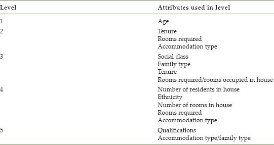
The construction of the model combines reconstruction of the population of small geographical areas with a two-stage process in which the desire to move house is evaluated. The ‘mover model’ (first stage) is regulated by a decision tree, which includes key household attributes such as age, family composition, social grade and ethnicity. Figure 5.1 shows the structure of the decision tree, while Table 5.1 identifies the attributes that contribute to branching at each of the levels shown in Figure 5.1. When the final choice in the decision tree has been reached, a movement probability is identified. The ‘choice model’ (second stage) mimics an evaluation process in which the influences of seven destination properties are combined. These elements are drawn using a combination of empirical research and evidence from the literature, comprising access to workplaces and schools, neighbourhood preferences for both ethnicity and social status, property size, tenure and distance (for more details, see Jordan, 2012; Jordan et al., 2012).
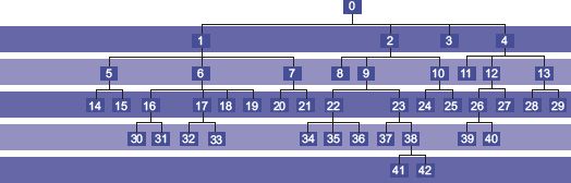
FIGURE 5.1 Decision tree structure
Source: Adapted from Jordan et al. (2012)
TABLE 5.1 Attributes used to differentiate the mover probability
The simulation is applied to a substantial part of Leeds with more than 100,000 individuals in which a social housing (publically owned and rented) programme has sought to create improved housing conditions for those on low income through a combination of new investment and changing tenure (e.g. stimulating private ownership of public housing stock). A number of scenarios were investigated, including the provision of new schools (found to provide a positive boost to the objective of increased mixing in the community) and the creation of a new transport corridor (found to have a negligible impact on social diversity).
Many of the extant applications of microsimulation to ‘what if?’ policy scenarios have a comparative static flavour – for example, they might compare equity of service provision to a population before and after the introduction of some change in the pattern of service delivery. However, this example has a much more genuine dynamic as housing moves are moderated through a ‘vacancy chain’ in which the decision to move simultaneously reduces the availability of property (as a new home is occupied) and increases it (through vacation of the current home). The decision rules introduce an interdependence between the decision-making units (e.g. if an affluent household moves into a neighbourhood of a lower social grade, then a marginal elevation of neighbourhood status takes place, and vice versa). This also starts to suggest an ABM flavour to the simulation, which has some similarities to well-known theories of neighbourhood segregation (e.g. Schelling, 1971) but much less stylised and with greater realism and practical potential.
Long-term strategic planning of infrastructure provision
A recent example of dynamic microsimulation applied to a strategic planning problem looking ahead more than 80 years has been provided in the work of Hall et al. (2014). This work has been undertaken as part of a bigger programme to explore alternative approaches to long-term transitions of infrastructure systems comprising transport, energy, water, waste and information technology. The long cycles of investment required for these crucial networks require that robust frameworks for future changes can be provided in both demographics and infrastructure demand, notwithstanding the obvious uncertainties and difficulties associated with this process (Beaven et al., 2014).
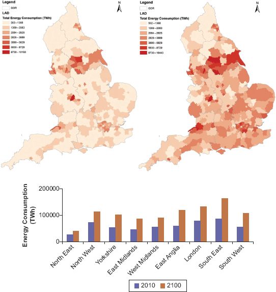
FIGURE 5.2 Long-term energy demand projection
In practice, the only sensible way to approach this problem is to adopt a scenario planning format. The work of Zuo et al. (2013) attempts systematic construction of a portfolio of scenarios across a full range of plausible future projections in the key demographic components of fertility, mortality and migration. The presentation of the model projections as a suite of microsimulated individuals and households provides a very flexible foundation for further modelling of the demand for infrastructure and the associated commodities – in fact, these authors implement a decision tree for attributes driving consumption which bears more than a superficial relation to the migrant generation process in Jordan’s housing model. As an example, Figure 5.2 shows how a long-term demographic projection, combined with baseline assumptions about energy consumption, can be used as a benchmark for changing patterns in future energy demand. The demographic projections can then be used as a basis for evaluation of alternative options and strategies for long-term infrastructure enhancement against a backcloth of both spatial and temporal disaggregation (Tran et al., 2014).
The process mechanisms for long-term demographic microsimulation of this type have been laid down in the work of Birkin et al. (2009). The flexibility of representing households, their constituent individuals and associated attributes is exploited as a means for driving transitions from one time period to another, through key sub-models which advance members of the population through cycles of migration, fertility, ageing, survivorship, household formation and fragmentation. In terms of the earlier discussion, the conceptual clarity and ease of a transition-based approach to the dynamic modelling task are preferred to the greater efficiency but somewhat more opaque event-based models.
Models of daily mobility
A novel approach to representing daily movement patterns in a simulated population has been proposed recently in the work of Harland and Birkin (2013a, 2013b). This work has some representational similarity to the movement models of Jordan as discussed above. Individual households and their constituent individuals are subject to a transition process that is driven by the spatial location and attributes of the entity. This example is distinguished, however, by the fact that moves are temporary rather than permanent, and are intended to represent cycles of movement against the daily, weekly and seasonal rhythms of demographic flux within a city region. Figure 5.3 shows the change in distribution of disposable income in the city of Leeds, UK, over the course of a normal working day.
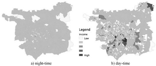
FIGURE 5.3 Simulated distribution of income
The potential value in model applications of this type is both evident and substantial (Birkin et al., 2013), for example in relation to problems of emergency planning, disease transmission, crime prevention or retail service provision. The procedures for capturing short-term movements in the population are not inherently difficult, although they do introduce some computational challenges in the execution of large numbers of decisions and also in monitoring and storing frequent shifts in the spatial position of each actor. Naturally simulating behaviour in a way that absorbs enough of the richness and complexity of movement and interactions in the ‘real world’ is a challenging programme. To date, the possibilities that have been adopted within the models combine elements of the mapping of different agents onto activity containers such as schools, hospitals and workplaces (in turn building on foundations laid in work such as that of Cockings et al., 2010); or consider the potential of social media for tracing movements and behaviours (Birkin et al., 2013). The greater potential of more wide-ranging datasets such as those maintained by mobile-phone-service providers such as Telefónica or Vodafone remain a tantalising but exciting proposition at the time of writing.
Technical architecture considerations
Abstraction
Ballas et al. (2006) point out synergies between the object-oriented programming paradigm and the conceptualisation of a dynamic microsimulation model into individual objects representing each individual micro-unit. However, representing individual micro-units as individual encapsulated programming objects has a trade-off against the memory and processing power required to run a model of considerable scale, such as for the whole of the UK. The Office for National Statistics (ONS) in the UK estimated the 2012 mid-year population to be approximately 63.7 million (ONS, 2013). Representing each UK individual with 63.7 million objects within a computer program would be a challenge, even allowing for the power of current technologies for computation.
Designing agent-based models, with their complex behavioural models, so that each individual is represented by an encapsulated object is logical. Each agent object can interact with other agent objects or the environment and react to input stimuli from either other agent objects or the environment independently. However, dynamic microsimulation models seldom require such detailed behavioural frameworks, with the outputs of events normally being defined by probabilistic or deterministic reactions derived from real-world observation. Taking the conceptual differences between ABM and dynamic microsimulation into consideration, it is potentially beneficial to consider the object currency (or level of abstraction) for a dynamic microsimulation model to be the processing framework, with the micro-units simply being data items passing through the framework. Figure 5.4 shows the difference between the two conceptual designs in diagrammatic form. Each object represents an individual micro-unit in Figure 5.4(a), with the behavioural framework and data reflecting the state of the micro-unit contained (or encapsulated) within each object. In contrast, Figure 5.4(b) shows a conceptual design where the micro-unit data are stored separately from the event-processing objects and are cycled through for events to take place.
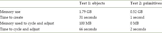
To exemplify the difference in processing efficiency, a simple test has been constructed. For benchmarking purposes the specification of the test computer is a MacBook Pro with 16 GB of random access memory and 500 GB solid state storage space running OS X Lion Version 10.7.5 on a 2.6 GHz Intel Core i7 processor. The test was run using the Java programming language through Netbeans version 7.3.1 and simply consists of storing 64 million randomly generated double-precision values in a single array. In the first test the numbers are stored as a ‘Double’ core language object in the Java programming language. In the second test the numbers are generated and stored as primitive values in the Java programming language (for a more detailed discussion of primitive values and objects in the Java programming language, see Schildt 2002). The first two rows in Table 5.2 show the amount of memory used and time taken to create and store the 64 million values for both tests. The bottom two rows show the extra memory used and time taken to cycle through the 64 million values, multiply the stored value by another randomly generated number and adjust the original value to be the result of the calculation. It is clear from the results in Table 5.2 that although considering the modelling approach from an event-processing perspective sacrifices the inherent logic of representing individuals as encapsulated objects, it has considerable advantages in storage capacity and processing time.
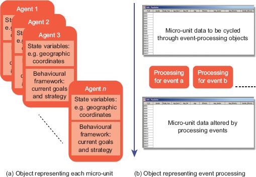
FIGURE 5.4 Alternative model architectures
The tests executed here are very simple representations of the two architectures considered but serve to highlight the significant differences between the two approaches. Adjusting the level of abstraction from the micro-unit to the event processing level provides significant scalability benefits.
TABLE 5.2 Test results for storage and processing efficiency
Events and actions
Orcutt (1957) outlined the need to represent interactions between demographic attributes from the micro level to effectively estimate and simulate how relationships between attributes develop and change over time and potentially space. The interrelated nature of events and attributes means that the dynamic microsimulation approach needs to have the flexibility to represent new events or interactions between events as they become apparent or important for the needs of the researcher. It is also important that the inclusion of new or modified events and relationships result in as little change to existing model architecture as possible, while considering that two seemingly separate events may result in very similar results. For example, consider a child leaving home for the first time and the breakdown of a marriage. These are two very different events potentially happening at different life stages of the individual. However, the action resulting from these two events is very similar, as one household unit effectively splits into two.
For these reasons, the programming architecture recommended here to represent events and actions is one similar to the architecture used for controlling user interaction with a graphical user interface. The graphical user interface typically consists of two parts: the first is something that the user interacts with, such as a digital button that generates events; the second is something that performs an action when notified to, an event handler. A third object is also created to hold information called the event. When the button is created, code is written to create an event object. The event handler is written to only handle the event type that it is concerned with, and it is attached to the button. When the button is pressed it broadcasts to anything listening that it has been pressed, creates the event object containing all the information important for the event and passes that to any objects listening. Any event handlers listening can then process the event. Figure 5.5 demonstrates this process diagrammatically.
This architecture promotes loose coupling between event generation and actions taken through event handling. As demonstrated in Figure 5.5, multiple event handlers can listen and action events created by a single generator, but also a single event handler can listen and action events created by multiple event generators. Additionally, the actions taken by the event handler may be dependent on the information contained in the event object which will be generated with specific information about the event, and likely information relevant to the micro-unit from which this event has been generated. Event handler 2 in Figure 5.5 could represent the example provided above where a new household is formed from both a marriage breakdown and a child leaving home. Event handler 2 actions the formation of a new household based on the information contained within the event object. Event generator 1 may be fired by a marriage breakdown, whereas a child leaving home may fire event generator 2. However, event handler 2 is ‘listening’ to both of these event generators and will action an event when either is fired.
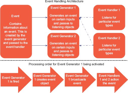
FIGURE 5.5 Event handling architecture and processing
Handling time
The advantages and disadvantages of transition-based and event-based models have been discussed above. It is proposed here that both of these approaches are accommodated. As Spielauer (2009a, 2009b) notes, dynamic microsimulation models are likely to require some elements of both approaches and that they are not mutually exclusive, citing the Australian DYNAMOD model as an example of a hybrid approach. It is proposed here that time is handled as a schedule broken down into time-steps. This is a similar approach to that adopted at George Mason University in the development of the MASON ABM toolkit:1 time-steps are the heart of the model, but there is also a scheduler that can be used to schedule events or actions. Here the model time-frame (time from start point to the end of the modelling time period) is specified alongside the time-step; for example, the time-frame is maybe 30 years and the time-step one month, resulting in a schedule of 30 × 12 = 360 time-steps. Events are then scheduled by the length of time to the event and placed onto the scheduler. However, the time-step mechanism also implements the event handling architecture, and it is therefore a straightforward matter to attach event listeners to event generators called at each time-step or at particular time-steps. In this way the model can work as a purely event-based model, purely as a transition-based model or as a hybrid, with some actions working from a schedule and some at each and every time-step.
Simple example
A simple example has been developed to test the architectural principles of event and time handling. The first stage of the process constructs a random population of 63.7 million individuals with a random age between 0 and 100 and a gender of either male or female, again randomly assigned. A schedule is created consisting of a time-frame of 30 years with a time-step of one week, which therefore consists of a schedule with 1560 time-steps. Births and deaths are randomly assigned to individuals and added to the schedule at a point in the future consistent with the numbers reported by ONS (2013) for 2012, 812,970 births and 569,024 deaths. Births are restricted to only occur to females aged between 15 and 45, while deaths randomly occur throughout the population.
Figure 5.6 shows a diagrammatic representation of events scheduled for each micro-unit. Once the schedule is formulated for each micro-unit, events are only processed at the scheduled points in time. However, if the interrelationship between events demands adjustment to future events, this can also be undertaken. Likewise, if an event occurring to one individual impacts another, the schedule for the secondary individual can be adjusted.
In our simple example, and Figure 5.6, the whole population is aged by one year after 52 time-steps, representing the 52 weeks in a year. Running this simulation uses 1 GB of memory and takes nine seconds to complete. The estimated population of the UK by 2042 using this very simple model is 73,114,216. The main aim of this example is to demonstrate the proposed model architecture functioning. It does not include critical features such as age-related mortality probabilities, fertility rates by age or any real representation of interactions between individuals or space. Parameterisation of the model is minimal, and it is accepted that as additional parameters and interactions are added, processing time and memory use will increase substantially. Despite these serious limitations, comparing the simple model output with a linear extrapolation of the ONS figures for births and deaths highlights an interesting point. Projecting the births and deaths 30 years into the future results in 569,024 × 30 = 17,070,720 deaths and 812,970 × 30 = 24,389,100 births. Combining these figures with the initial start population 63,700,000 + 24,389,100 – 17,070,720 results in a population estimate of 71,018,380. The simple dynamic microsimulation has captured a potential increase in the population greater than that resulting from a linear extrapolation. This is simply the result of births outstripping deaths and an expanding number of females eligible to give birth, producing a non-linear expansion of the population. This supports Orcutt’s (1957) suggestion that modelling at the micro-unit level naturally captures relationships between attributes that are difficult or even impossible to represent using aggregate data alone.
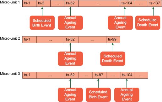
FIGURE 5.6 Diagrammatic representation of time handling
Discussion
Advances in both theory and computation have allowed significant extension of the ideas originally presented by Orcutt (1957). One powerful innovation that has been facilitated is the representation of individual micro-unit actors as software objects within social science models (Ballas et al., 2006). Nevertheless, alternative modelling architectures are open to researchers, as Crooks and Heppenstall (2012) note. An exemplification of this point was demonstrated above. Representing individuals as computer objects proved to be computationally much more onerous than holding and processing the same information as a series of indexed individual data items. Evidently, a trade-off exists between model efficiency and the logical representation of the individual micro-unit that needs to be considered when a model is in the design phase. Design questions should be asked including:
1. What are the scalability requirements for this simulation exercise?
a. the number of actors in the model;
b. the time-horizon for the simulation.
2. Is complex behaviour an integral part of the research?
3. What level of interaction is required?
a. actor to actor;
b. actor to environment;
c. environment to actor.
These types of questions help ascertain the modelling approach most suitable for the research exercise. Dynamic microsimulation and ABM have many similarities, and it is becoming increasingly difficult to definitively select one approach to use in a research project. Some suggestions have been made above relating to where the interface between dynamic microsimulation and ABM lies. One suggestion is that agent-based models have bidirectional interaction between the digital environment and the micro-unit actors, whereas dynamic microsimulation has unidirectional interaction with actors unable to influence the environment. However, this distinction may not always be clear-cut. The work of Jordan (2012) represented migrations in a dynamic microsimulation model through interactions with housing stock in the digital environment. The migration of one micro-unit is seen to impact on the decisions of other micro-unit actors on where to locate as the available housing stock in the environment has changed. The interaction here was clearly bidirectional, so elements of this model might equally well be described as agent-based. Since the model also clearly has many of the traits of a transition-based dynamic microsimulation model, perhaps an overall characterisation as an hybrid model would be most appropriate. Increasingly it may be less critical to think in terms of model definitions as ABM and dynamic microsimulation, but rather as a continuum between approaches (e.g. Wu et al., 2008).
Recently microsimulation, ABM and other modelling approaches not discussed here such as cellular automata have been described under the umbrella term ‘individual-level’ models. As research progresses and computational power increases, the distinctions between different modelling approaches will become ever more difficult to discern and arguably less important. In 50 years, perhaps less, computational power may well be at a level to enable models with millions of actors each with complex behavioural frameworks and multi-directional interactions. Such models could be relatively easily achievable for researchers to access as modelling toolkits become more advanced.
A future scenario of this kind is not inconceivable, considering that 30 years ago the desktop computer and the internet were still embryonic research projects. The pace of progress is increasing, not slowing; therefore it is entirely likely that such complex models of human society may well be achievable within the working lifetimes of the current generation of researchers. Examining the differences between modelling approaches to enable closer integration is perhaps one of the more exciting prospects for researchers in the social science modelling arena. There is every likelihood that increasingly massive portfolios of behavioural data at a variety of spatial and temporal scales (‘Big Data’: Birkin, 2013) will provide a further impetus to the pace of change. However, in a research world where ‘big data’ and individual level models may well proliferate, considerations about model evaluation and validation will become increasingly important and significantly more challenging than they already are. Where and how these important requirements for social science modelling will fit in with individual-level models is a question yet to be resolved. And how sense can be made of the huge volumes of data that will be produced by such models is an equally significant challenge for future research. These questions may be the real future challenge as the integration of modelling approaches appears to be naturally occurring as computational power and model accessibility progress.
FURTHER READING
A recent overview of microsimulation approaches is provided by Tanton and Edwards (2013). For a a real and detailed example of the use of agents within a dynamic microsimulation, see Wu et al. (2011). Harland (2013) is a practical manual which presents software codes, sample data sets and easy-to-follow instructions for readers wishing to develop their own microsimulation models. Finally, for an authoritative introduction to the application of microsimulation as a technique for demographic modelling, see Van Imhoff and Post (1998).
1http://cs.gmu.edu/~eclab/projects/mason/.
All materials on the site are licensed Creative Commons Attribution-Sharealike 3.0 Unported CC BY-SA 3.0 & GNU Free Documentation License (GFDL)
If you are the copyright holder of any material contained on our site and intend to remove it, please contact our site administrator for approval.
© 2016-2025 All site design rights belong to S.Y.A.