Geocomputation: A Practical Primer (2015)
PART II
EXPLORING MOVEMENTS IN SPACE
6
SPATIO-TEMPORAL KNOWLEDGE DISCOVERY
Harvey J. Miller
Introduction
The transformation from a data-poor to a data-rich environment is the most profound event in the history of geography and earth science. For most of history, we invested a tremendous amount of resources and time, and quite often human lives, to tease small trickles of geographic data from the environment. Those trickles have become floods due to the rise of sensing systems and location-aware technologies such as satellite and airborne remote sensing, the global positioning system, mobile phones, sensor networks and georeferenced social media.
Much of the data torrent is spatially referenced and time-stamped (Rohde and Corcoran, Chapter 7). These ubiquitous, ongoing spatially and temporally referenced data flows are potentially revolutionary since they allow us to capture spatio-temporal dynamics more directly (rather than inferring them from periodic snapshots) and at multiple spatial and temporal scales. Also, since the data are collected on an ongoing basis, they can capture both mundane and unplanned events, allowing data-rich, naturalistic analysis that can lead to new discoveries about the dynamics of people, cities, societies and the environment (Miller and Goodchild, 2014).
Our statistical and spatial analysis techniques are to a great extent not designed to find patterns and information that may be hidden in spatio-temporal data streams and mobile objects data. These techniques are confirmatory: they require the researchers to hypothesize variables tied together in a highly specific relationship. Statistical testing can only tell if the postulated model does not fit the data; it cannot suggest alternatives (Guo and Mennis, 2009). While confirmatory methods have their role, they are not well suited to exploring massive spatio-temporal data: the number of possibilities is too large to explore in this tedious manner.
Massive spatio-temporal datasets require new exploratory methods: techniques that can efficiently discover patterns hidden deep within their stuctures. While this information may be tentative, it can enhance the initial stages of the scientific process by generating new insights and novel hypotheses to be tested using confirmatory techniques (Gahegan, 2009; Gahegan et al., 2001; Miller, 2010)
It is common to use the term ‘data mining’ to describe the process of exploring databases for novel, unexpected patterns. Data mining is the application of low-level algorithms and techniques to search for hidden patterns in data (Alexiou and Singleton, Chapter 8). However, this is only one part of a broader, higher-level knowledge discovery process that requires interlinked decisions about how to prepare and manage data, the identification of those properties and features to be explored, the selection of data-mining techniques and interpretation of the results in light of the analyst’s background knowledge about the real-world domain. Knowledge discovery is a complex, intricate process that requires human-level intelligence for guidance.
This chapter discusses processes and techniques involved in discovering new spatio-temporal knowledge from spatially referenced and time-stamped data, including data on moving objects. It presents background material, and includes discussion of those issues surrounding the processing of spatial, temporal and moving objects data to extract properties of interest. It also includes strategies for building and populating a data warehouse or the database designed to support such analysis and exploration. It discusses major methods for exploring and mining spatio-temporal data, including data cubes, clustering, association rules, sequence mining, mining collective patterns and visual analytics. The chapter concludes with some summary comments.
Processing spatial and temporal data
Spatial, temporal, and mobile objects data are potentially interesting since proximity in space and coincidence in time affect many human and physical phenomena. Spatial relations are measures of proximity in space. Major classes of spatial relations are set-oriented, topological, directional and metric relations (Worboys and Duckham, 2004).
Set-oriented relations conceptualize spatial relations between objects using set theory concepts such as intersection, union, difference and complement. Topological relations focus on connectivity, interior, exterior and boundary relationships between spatial objects (Egenhofer and Franzosa, 1991). Directional relations between spatial objects include cardinal (e.g. ‘the factory is west of the neighborhood’), object-centered (‘the neighborhood is behind the factory’) and ego-centric directions (‘the factory is on your left’). The major type of metric spatial relation is distance, such as Euclidean or network-based distance.
Temporal relations are measures of coincidence. The number of possible temporal relations is also surprisingly large: there are 13 possible temporal relations between two time intervals, including meets, equals, starts and finishes(Allen, 1984). Time also does not need to be linear: cyclical and branching real-world timelines are also possible. Natural cycles such as seasons are cyclical, and branching time can represent different versions of the past or possible futures.
With respect to a moving object, we can distinguish among movement properties based on temporal scale. Moment properties include its time, location, direction, speed, acceleration/deceleration and accumulated travel time and distance at a given instant in time. Interval-based properties include its geometric share, traveled distance, duration, the dynamics and distribution of speed and direction, and the ordering of these properties over a sub-segment of a moving object’s trajectory in space with respect to time. Episodic properties are movement properties associated with an external event in space or time; an example is people within a park during lunch. Global properties are those defined for the entire space–time trajectory traced by an object (Andrienko et al., 2008b; Laube et al., 2007).
A challenge in exploring spatio-temporal data is that spatial and temporal relations and properties are usually not explicitly stored in the database. A database will only store the locations and footprints of the objects in a spatial reference system, and time-stamps corresponding to sample times, events in the real world and database transactions (e.g. when a change was recorded in the source database). Spatial and temporal properties must be computed from the data based on the location and geometry of the spatial objects as well as time-stamps.
Processing spatial data is computationally demanding because it is often voluminous due to its geometry. Furthermore, many spatial algorithms require computational geometry procedures that are time- and storage-consuming. A common database and tool design question is whether to conduct operations involving spatial data before the data-mining process (as a so-called precomputation stage) or ‘on the fly’ during the process (Andrienko et al., 2006). The former case requires a great deal of overhead and requires these calculations to be updated if the database is updated. Some of these extracted properties and relations may not be needed. The latter strategy can, however, slow the data mining, causing great harm to the exploratory process which needs to be fast and nimble to maximize the human–computer interaction experience.
Another issue in mining spatio-temporal and moving objects data is the spatial resolution or temporal granularity of the data. There is a trade-off between the interest level and the support strength for patterns at different levels of resolution and granularity. More interesting patterns are likely to be discovered at the highest resolution and granularity levels, but the smaller number of database cases at these levels means that data support may be low, meaning that confidence in these patterns will also be low. Conversely, there is likely to be large data support at coarser resolutions and granularity, but these patterns are not likely to be interesting (Andrienko et al., 2006). It is also critical to keep in mind that the problem of artificial or ‘modifiable’ units of analysis in both space and time can also greatly affect the results of exploratory analysis just as it does in confirmatory analysis (Long and Nelson, 2013).
A challenge associated with processing moving objects data is that the object’s movement pattern is not directly available: location-aware technologies only capture a sequence of locations at discrete moments in time. There are several ways to capture this location sequence (Andrienko et al., 2008b; Ratti et al., 2006). The simplest and most common manner to reconstruct an object’s movement from a temporal sequence of recorded locations is through linear interpolation. This assumes that the object followed a straight line between recorded locations. We can deal with the location uncertainty that results from undersampling by constructing uncertainty regions that delimit the locations where the object could be, based on how fast the object could move and the length of the time interval (Kuijpers and Othman, 2009; Pfoser and Jensen, 1999).
Data warehousing
Data explored and analyzed during the knowledge discovery process are often integrated from disparate sources and stored in a specialized database known as a data warehouse (DW). This is usually an integrated archive or repository of other databases. It may be drawn from a project or organization’s operational database that supports day-to-day activities. However, it also need not be internal to a project or organization: it may consist of views into external databases existing on remote servers and accessed using the internet. Data accessed remotely may be published versions of internal databases, such as data selectively released on the web for public consumption by governments, business and organizations. It also may be data ‘scraped’ from the web and social media through application programming interfaces, including volunteered and shared data from citizens. Therefore, a DW may be a heterogeneous collection of authoritative, clean data and informal, messy data.
Extraction, transformation, and load (ETL) functions perform the tasks required to copy data from source databases, making them more usable, and store them in a DW. ETL functions include decoding and encoding data, merging/splitting of attributes, data aggregation and summarization, cleansing through removal of errors and outliers, and data smoothing. ETL for spatial and temporal data requires wide-ranging expertise. For example, the system must ensure that source data are topologically correct and respect spatial and temporal integrity constraints, and that the overlay of these data with other spatial data is also topological correct and coherent with respect to updates. There are also problems of georeferenced data with different map scales and referencing systems, objects and timelines represented with different spatial and temporal granularities and semantic heterogeneity (e.g. the definition of ‘city’ or ‘mountain’ may vary with location). Mobility data may be collected using different methods and at different levels of granularity; these data may need to be resampled prior to integration. Given this range of expertise, it is unclear that spatial ETL functions could be executed automatically without human intervention; for example, software ‘wizards’ that ask users questions at crucial decision points in the ETL process (Bédard and Han, 2009).
A DW has different design objectives than standard databases. Operational databases are designed to support transactional processing: editing, updating and other database activities by multiple users. This usually involves avoiding repeated data and minimizing the number of logical connections among data items in the database design. Since a DW is an archive we do not need to worry about transactions and instead can design it to support analytical processing. Therefore a DW will have repeated and highly interconnected data to reduce the effort required to search and link data during exploratory analysis. This means that a DW may be much larger than the combined volume of the individual source databases (Miller and Han, 2009).
Spatial data warehouses (SDW) and trajectory data warehouses (TDW) must have support for spatial and temporal data storage and access methods such as spatial, spatio-temporal and mobile objects database indexes (Bédard and Han, 2009; Pelekis et al., 2008). Given the complexity and volume of spatial, temporal and mobility data, a design issue is also which measures to pre-compute and store in the database, as discussed above. There are three major strategies for SDW. First, we could simply store spatial data with no pre-computed spatial measures. A second strategy is to pre-compute and store a rough approximation of the spatial measures, such as those based on minimum bounding rectangles rather than the spatial objects themselves. A third strategy is to selectively pre-compute some spatial measures (Papadias et al., 2002; Shekhar et al., 2001; Stefanovic et al., 2000). With TDW we also have the choice of whether to not pre-compute any trajectories, pre-compute a limited portion of an individual trajectory, an entire trajectory or all trajectories (Pelekis et al., 2008).
Exploring and mining spatio-temporal data
The above discussion concerned how spatio-temporal data can be integrated within SDW and TDW. In this section, this discussion is expanded to consider a series of common methods that are used to both explore and mine spatio-temporal data. The methods discussed have been selected as they are commonly used; however, within this topology, there is diversity both within classes, and at the boundaries between different methods.
Space–time cubes
A data cube is method for organizing and managing database summary measures for querying, visualization, or inputs into data mining techniques. A data cube is a multidimensional extension of a spreadsheet: it is a logical arrangement of data measures that allows quick summaries and cross-tabulations at different levels of aggregation. Summary measures can include distributive functions (e.g. count, minimum, maximum, sum), algebraic functions(e.g. average, standard deviation), or holistic functions (e.g. median, mode, rank). These summary measures can be pre-computed and stored to increase query performance (Gray et al., 1997; Han and Kamber, 2012; Rivest et al., 2005).
Figure 6.1 illustrates a data cube. Given a measure (such as ‘sales’) and dimensions of interest (such as ‘item’, ‘location’ and ‘time’), the corresponding data cube is the three-dimensional data lattice shown. A data cube will store the measures as well as their summaries at all possible levels of aggregation (e.g. total sales by item and location, total sales by location and total sales). We can also manipulate and query the data cube in several ways. A slice of the data cube is a selection based on a single dimension: for example, we could select all sales data for 30 November 2012. Dicing creates a sub-cube by selecting data based on conditions for two or more dimensions: for example, we could select all sales for all items in Chicago on 30 November 2012. We can also perform a roll-up (aggregation) operation that removes a dimension from the cube. For example, if we rolled up the cube in Figure 6.1 by removing the time dimension, we would have sales for all items by location for all times. We can also disaggregate or drill down the data cube by adding an additional dimension, such as ‘customer type’ (Han and Kamber, 2012).
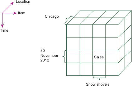
FIGURE 6.1 A three-dimensional data cube
Concept hierarchies can enhance roll-up and drill-down operations on data cubes. For example, we might provide a concept hierarchy for the location dimension with the levels (from lowest to highest) City < State/Province < Country. Similarly, we could have a concept hierarchy for the time dimension with the levels Date < Week < Month < Season < Year. Concept hierarchies provide a different and often richer way to aggregate and disaggregate data for exploration (Han and Kamber, 2012).
A spatial data cube or map cube is a data cube for spatially referenced data. A map cube can have three types of spatial dimensions: non-geometric (nominal categories, such as ‘Chicago’ in Figure 6.1), geometric (having spatial objects at all levels) and mixed (spatial objects associated with some levels of aggregation but nominal spatial references at other levels; an example is spatial objects at the state/province level but nominal spatial references at the national level). A map cube can also contain spatial aggregation operations, including spatial distributive functions (such as a minimum bounding box for an object or object collection, union and intersection among spatial objects), spatial algebraic functions (such as centroid and center of gravity) and spatial holistic functions (such as nearest neighbor) (Bédard and Han, 2009; Rivest et al., 2005).
A space–time attribute cube contains spatial, temporal and non-spatial dimensions (Guo et al., 2006). Space–time cubes contain only spatial and temporal dimensions with different levels of granularity. An example of a space–time cube is a traffic cube: a space–time cube for traffic data (Lu et al., 2009). Figure 6.2 shows a space–time plot for traffic counts based on slicing the space–time cube for day of week by time of day for the week corresponding to the American Thanksgiving holiday in the year 2003. The impact of the holiday on Thursday can clearly be seen in the plot, as well as the transition into the unofficial shopping holiday on Friday (Song and Miller, 2012).
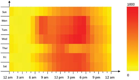
FIGURE 6.2 Visualizing a slice of a space–time cube: time of day versus day of week for traffic count data
A large number of data-mining techniques can be applied to spatio-temporal data after they have been prepared, stored and organized. Major classes of data-mining techniques include clustering, association analysis, classification, generalizations, trend detection and outlier analysis (see Andrienko et al., 2008a; Fayyad et al., 1996; Miller and Han, 2009). Most of these techniques have been extended to spatio-temporal data, typically focusing on algorithmic aspects and fast approximation techniques for calculating spatial and temporal relations and properties for inclusion into data mining techniques (Nanni et al., 2008). In the remainder of this methods section, we will focus on techniques that are particularly well suited for spatio-temporal and mobility data.
Spatio-temporal clustering
Cluster analysis involves sorting a set of objects into a smaller number of groups consisting of members that are similar (see Alexiou and Singleton, Chapter 8). In standard (non-spatial) clustering, similarity is based on attribute values. With spatial and temporal data, similarity may also include spatial proximity and/or temporal coincidence. There are numerous cluster analysis techniques. Partitioning methods divide a dataset into a smaller set of groups such as that each group has at least one member and each item belongs to exactly one group. Hierarchical methods start from the top down (divisive) or bottom up (agglomerative) to build a multi-level system of clusters. Densitymethods grow clusters by adding objects as long as the density of objects within a defined neighborhood meets a minimum threshold. Grid methods divide the object space into a grid and cluster based on that structure. Density- and grid-based methods can be effective for spatial and temporal data since they can discover arbitrarily shaped clusters as opposed to compact, spherical shaped clusters as in partitioning and hierarchical methods (Han et al., 2009). Self-organizing maps are another clustering method based on neural networks that has also been shown to be effective for spatio-temporal data (Agarwal and Skupin, 2008).
Clustering moving objects data requires measuring similarity between space–time trajectories. Shape-based similarity measures focus only on the geometry of the trajectories, ignoring sequence and time. Euclidean distance is intuitive and easy to calculate, but sensitive to noise and outliers. Hausdorff distance is the maximum of the minimum distances between two paths but can be misleading since it does not take into account temporal sequence. Figure 6.3 illustrates a case where two paths have a low Hausdorff distance although the two mobile objects are unlikely to have been proximal in space at any time (Yuan and Raubal, 2014).
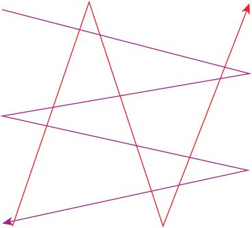
FIGURE 6.3 Two trajectories with a low Hausdorff distance despite the lack of spatio-temporal proximity between the mobile objects
Time-based methods include Fréchet distance, dynamic time warping and longest common subsequences. Unlike the Hausdorff distance, the Fréchet distance takes into account the sequence of locations in the path and is therefore better suited to mobile objects (Maheshwari et al., 2011). Dynamic time warping measures the similarity between two sequences or trajectories, based on the effort involved to stretch or compress time to get the sequences to match. Least common subsequence measures similarity based on the length of least common subsequence between two sequences (Dodge et al., 2012; Nanni et al., 2008; Yuan and Raubal, 2014).
Edit-distance functions measure similarity between sequential patterns based on the cost of the insertion, deletion and substitution operations required to transform one sequence into the other. In traditional sequence pattern similarity measurement the cost of each operation is set constant, but for spatio-temporal sequences we can measure the operations costs based on the spatial and temporal relations between the corresponding trajectory data points. Yuan and Raubal (2014) develop edit-distance similarity measures for comparing mobile-phone trajectories based on spatial, temporal and spatio-temporal distance of each point from the trajectory’s centroid. They also develop an edit-distance function constrained by time-windows corresponding to semantic time periods (such as ‘morning’ and ‘evening’).
Spatio-temporal associations
Association rule mining involves searching data to discover conditions occurring together frequently. Association rules are of the form X ⇒Y(s%, c%) where X and Y are conditions that occur together and (s%, c%) are the levels of support and confidence for the rule; these correspond to the empirical probabilities P(X ∪ Y) and P(Y | X), respectively. For example, the spatial association rule
Is (School) ∧ near (Sports Center) ⇒ near (Park) (2%, 55%)
means that 55% of schools that are near a sports center are also near a park, and this occurs in 2% of the items in the database (Han and Kamber, 2012).
Association rule mining requires finding all itemsets in the database that occur together based on a user-defined support threshold and then generating association rules from that subset based on a user-defined confidence level. Mining for spatial, temporal, and spatio-temporal association rules is complex since finding associations requires computing spatial proximity and temporal coincidence relations from the data (Mennis and Liu, 2003). A strategy for managing this complexity is filter-and-refine: first mine the full database using approximations of the spatial objects such as minimum bounding rectangles or convex hulls; then refine these results by mining the detailed spatial objects in the smaller candidate dataset, removing the false positives (Han and Kamber, 2012).
Verhein and Chawla (2008) develop space–time association rules (STARs) that describe how objects move among a set of regions over time. STARs apply to specific time intervals and describe how objects move among a set of regions during those intervals. Regions can be any shape or size. An example is the rule:
Is(Office worker) ∧ outside (City) ∧ time(Night) ⇒ inside (City) ∧ time (Morning)
In other words, office workers who are outside of the city at night tend to head into the city in the morning. They also extend the concept of coverage and support to space and time by considering the lengths and sizes of the time intervals, spatial regions and objects described by the rules. They develop rules for empirical concepts such as stationary regions and high traffic regions, with the latter consisting of sources, sinks and thoroughfares.
Sequence mining
Closely related to association rule mining is sequence mining: searching for patterns in time or other sequences. Most sequential mining techniques concentrate on symbolic patterns, searching the database for events (symbols) that occur frequently together. The search is similar to association rule mining, but is based on three search parameters: the duration of the time sequence, the event window or time-horizon for considering events as temporally coincident, and the time interval between events.
Periodic pattern mining is a type of sequence mining that searches for recurrent patterns. These can include: (i) full periodic patterns where every point in time contributes either exactly or approximately to the cyclic pattern (e.g. all days of the year approximately contribute to the season pattern); (ii) partial periodic patterns that are true for some but not all points in time (e.g. a person may visit a particular coffee house at 7:00–7:30 a.m. every Monday through Friday but display no other regular activity patterns); (iii) cyclic or periodic association rules that associate events that occur periodically (e.g. a busy afternoon in a restaurant implies a busy evening rush). Both sequential and periodic mining can be conducted as a database search in a manner similar to association rule mining (Han and Kamber, 2012).
Extending sequential and periodic mining techniques to mobile objects data requires solving two sub-problems: (i) how to detect the periods in complex movement patterns; (ii) how to mine the period behavior. A strategy is to search for reference spots or locations that are repeatedly visited by the objects and then mine for recurrent movement patterns between these reference spots (Li et al., 2012). Bleisch et al. (2014) combine these techniques with a conceptual framework regarding the possible causal relations between states and events in the world to infer causal and causal-like relationships between movement patterns of mobile objects with associated measures of support and confidence.
Mining collective patterns
Another important set of patterns associated with moving objects data are collective motion patterns. These focus on individual object movement patterns within the context of a larger group of mobile objects (Long and Nelson, 2013). Distance-based measures search for collective patterns such as flocks by searching for moving objects that are densely connected in space given user-defined distance and time thresholds (Gudmundsson and van Kreveld, 2006). Laube et al. (2005) develop a relative motion (REMO) approach that considers the individual directions in a group of moving objects to detect collective patterns such as flocking, leadership, convergence and encounter. Gudmundsson et al. (2007) improve the efficiency of the REMO approach using techniques from computational geometry.
Visualization and visual analytics
Visualization is a powerful strategy for leveraging human visual acuity to help make sense of data and discover patterns and anomalies in spatio-temporal data. Visualization is particularly essential for analyzing processes unfolding in geographical space with respect to time. The heterogeneity of geographic space and the variety of properties and relationships within it cannot be adequately represented in algorithmic processing, exploration, and analysis of spatio-temporal data. Visualization facilitates the derivation of knowledge from spatio-temporal data by leveraging the human analyst’s sense of space and place, tacit knowledge of their inherent properties and relationships, and space/place-related experiences (Andrienko et al., 2008a).
More than just another exploratory technique, visualization is also a powerful method for integrating and enhancing all aspects of the spatio-temporal knowledge discovery process from data management through to guiding the exploration process, interpreting the results and constructing new knowledge (Gahegan, 2009). Visual analytics is the science of data-driven reasoning facilitated by interactive visual interfaces to data management and analysis techniques (Thomas and Cook, 2004). Visual analytics is more than just information visualization: while visualization provides insights into data, visual analytics provides insights into how we process data during exploration and analysis (Keim et al., 2008).
Visual analytics for spatio-temporal data includes techniques such as attribute plots, time plots, space–time cube operations, methods for data selection and data-mining techniques such as clustering; all linked together though interactive visual interfaces with the map as the central metaphor (Guo, 2003, 2009; Guo et al., 2006). Visual analytics for moving objects data includes linked techniques for analyzing and comparing entire trajectories, variations of properties within trajectories, synoptic visualization and analysis of the moving objects as a whole, and investigating movement within the spatio-temporal context in which it occurs (Andrienko et al., 2013).
Conclusion
We have entered an unprecedented era for research in geography and earth sciences. The world is awash with spatially and temporally referenced data flowing from remote sensing systems, location-aware technologies, embedded sensors and social media. Confirmatory techniques are not well equipped to explore these massive spatio-temporal databases and to discover information hidden in them.
Spatio-temporal data-mining techniques applied within the broader knowledge discovery process have the potential to generate new insights into human, physical and linked human–physical systems. Spatio-temporal knowledge discovery is the intricate process of preparing, managing and exploring massive spatio-temporal databases to generate novel geographic knowledge. Spatio-temporal data offer unique challenges to knowledge discovery due to the volume and complexity of these data as well as the implicit nature of spatial and temporal relations and properties within spatially and temporally referenced data. However, recognizing the value of spatio-temporal data, a large and vibrant interdisciplinary research community has emerged over the past two decades to meet these challenges. New methods and techniques for integrating and managing spatio-temporal and moving objects data are being developed, as well as techniques that can exploit the spatial and temporal properties of these data to generate new geographic knowledge.
A new data-driven scientific geography is emerging in response to the wealth of spatially and temporally referenced data, flowing from sensors and people in the environment, as well as capabilities for extracting new knowledge from these data. While this is very promising, perhaps revolutionary, there are some cautions. Data-driven knowledge is idiographic – contingent on particular places and times – while science seeks nomothetic (general, law-like) knowledge. We must be cautious about where this research is occurring – in the open light of scientific peer review and reproducibility, or behind the closed doors of private-sector companies and government agencies. Privacy is a concern not only as a human right, but also as a potential source of political and societal backlash that will curtail data-driven research. Finally, we must remember that data should not make decisions for us. Data should support but not replace decision-making by intelligent and skeptical scientists (Miller and Goodchild, 2014).
FURTHER READING
Hey et al. (2009) is a collection of short, empirically oriented essays about how data-driven science will change fields ranging from earth science to medicine. Miller and Han (2009) is an edited collection of chapters describing spatial and spatio-temporal data-mining methods. Several chapters provide a basic review of methods such as spatial data warehouses, map cubes and spatio-temporal clustering.
All materials on the site are licensed Creative Commons Attribution-Sharealike 3.0 Unported CC BY-SA 3.0 & GNU Free Documentation License (GFDL)
If you are the copyright holder of any material contained on our site and intend to remove it, please contact our site administrator for approval.
© 2016-2026 All site design rights belong to S.Y.A.