Geocomputation: A Practical Primer (2015)

PART II

EXPLORING MOVEMENTS IN SPACE

7

CIRCULAR STATISTICS

David Rohde and Jonathan Corcoran

Introduction

Geocomputation involves the analysis of data in many forms, including real numbers that might include information on distances or times, counts derived from census tables, or categorical variables drawn from survey data, to name only a select few. The analysis of these datasets requires the use of statistical methods based upon distributions with appropriate support, for example the normal distribution which has support over the real numbers (i.e. negative or positive values) and the Poisson distribution which has support over the natural numbers (i.e. count data, see Nakaya, Chapter 12). In this chapter we consider another type of data of interest to geographers: namely, angular or directional data.

Angular quantities are real numbers but with bounded support on the interval [0,2π] (radians) or [0,360] (degrees) and the unusual property that quantities near the extremes of 0 and 2π are in fact close. The consequences of these unusual properties are that statistical methods that apply to real data can give very misleading results when applied to angular datasets. It is from these unusual properties that the sub-discipline of circular statistics was born; Fisher (1995: 1) described it as a ‘curious byway of statistics’, with origins dating back to the mid-eighteenth century (Bernoulli, 1808). Early applications of circular measures were employed to demonstrate that the orbital planes of planets in the solar system could not be aligned by chance (Mardia, 1975), and Florence Nightingale (1858) developed the coxcomb (or rose diagram) to visually depict the efficacy of improved sanitation in hospitals during the Crimean War. A number of books have since been devoted to the topic of circular statistics; of particular note are Fisher (1995) and Jammalamadaka and Sengupta (2001).

The importance of circular statistics to analytical geography in the examination of spatial phenomena is twofold: first, as a technique to analyse direction (e.g. direction of travel); and second, to investigate the temporal dynamics of phenomena (e.g. time of day or day of week, see Figure 6.2 on page 103 for a visual approach). In both cases circular statistics have a potentially important role to play in uncovering directional and temporal dynamics of spatial phenomena. The focus of this chapter will be on the examination of directional dynamics. In general, the previous research on using directional data has tended to focus on data with no explicit spatial frame in which applications in geology and biology have been particularly prevalent. Despite the general lack of application of circular statistics in geography, the potential that such techniques hold in terms of their capacity to augment the geographer’s analytical toolbox is significant in permitting new ways to analyse and visualise spatial data. In bringing this new approach to the study of geographical datasets, new questions can be posed that may include derivatives of the following (taking commuting data derived from the census by way of example):

1. What is the mean direction of commuter travel, and how does this mean direction vary from one region to the next?

2. Does the mean direction of commuter travel of any one travel zone differ significantly by gender and mode of travel?

3. Have there been observable shifts in mean directions of commuter travel between census waves, and, if so, how do these relate to changes in urban form?

With the general thrust of these questions in mind, this chapter aims to encourage readers to think about their own datasets and how these questions may be reformulated with these different contexts. Furthermore, this chapter aims to encourage readers to experiment with the analysis of circular data using pre-existing software libraries such as Berens (2009) for MATLAB or the circular package for R (Agostinelli and Lund, 2011).

The remainder of this chapter is organised as follows. First, we outline how descriptive statistics analogous to the mean and variance can be used to summarise circular or angular data. We then present the von Mises distribution as one of the most useful circular distributions, but also wrapped distributions as another very flexible way to define a probability distribution of a circular quantity. These discussions are then extended to develop semi-parametric and non-parametric statistical models, alongside the statistical testing of circular quantities. The remainder of the chapter is concerned with a case study analysing the direction of travel utilising data derived from a bus electronic ticketing information system in Brisbane, Australia. Concluding remarks are then made alongside further reading.

Descriptive statistics

There are two ways to represent an angle, using either polar coordinates θ or a vector r constrained such that |r|=1; the latter method is also useful in considering angles on spheres, a topic that is beyond the scope of this chapter. The two methods are related in the following way:

The most basic of questions we might consider for a collection of angular data θ₁,…,θ_n is to compute the mean. It is rather obvious that the conventional mean will fail to take account of the fact that 0 and 2π are identical and that values around this region are in fact close, the so-called cross-over problem. An alternative approach is to compute the average based upon rectangular coordinates r₁,…,r_n, i.e. through which the angle can be recovered by converting this quantity back to polar coordinates. This is achieved using

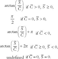
The rather complicated conditions in this equation are due to the fact that the ratio cannot distinguish between cases such as and both negative and and both positive (or one positive and the other negative). The operation is common enough that the function arctan2(,) is often defined as above (or more commonly, as a slight variant with support over [−π,π]) and is available in many programming languages, including MATLAB and R.

It is noteworthy that unlike the individual observations r₁,…,r_n which all have magnitude 1, the statistic usually does not; in fact, a quantity that is useful in measuring the spread is given by 1 – , and is sometimes referred to as the circular variance. The circular variance ranges from 0 to 1. An intuition for this statistic can be gained by imagining that r₁,…,r_n are all identical, in which case R lies on the unit circle and = 1, and as a consequence the circular variance is 0. Alternatively, if r₁,…,r_n are uniformly spread, these cancel each other out exactly, then and the circular variance is 1; also note that in polar coordinates the mean angle is in this case undefined. An undefined mean is an interesting special case that occurs with circular statistics, but not linear statistics. While it might seem strange to have the mean undefined, it does makes intuitive sense that a distribution that is uniform over all angles has no mean.

Circular distributions

The normal or Gaussian distribution is fundamental to linear statistics and has support on the real numbers. In order develop statistical methods for circular data it is useful to consider distributions with support on the interval [0,2π]. One of the important properties of the normal distribution is that it has sufficient statistics, i.e. it is possible to summarise all of the information about the data likelihood from a sample from a normal distribution using just the sample mean and sample variance. The distribution for circular quantities that has sufficient statistics is the von Mises distribution, which has the form

for polar coordinates in radians, or

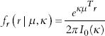
for rectangular coordinates (often referred to as the Fisher–von Mises distribution). The latter distribution can easily be generalised to spheres and hyperspheres. The normalisation of these probability densities requires the use of a Bessel function which is available in most programming libraries, although direct use of this function is often made unnecessary by the use of circular statistics libraries available for many programming languages. A series of scripts accompany this text in MATLAB, and are provided in order to demonstrate how to reproduce these results.

A histogram of circular data is shown in Figure 7.1. For this dataset, and = 0.2518π or 45.3 degrees. This estimate of the average angle gives a good representation of the peak in Figure 7.1. The linear mean is 0.6459π or 116.3 degrees. The failure of the linear mean to identify the mode of the distribution gives an illustration of the change-point problem. The change-point problem refers to the fact that 0 and 2π are identical and points on either side of these values are in fact close.

A fit of the von Mises distribution found using numerical methods results in the parameter estimates µ = 0.2518π and K = 2.2914.

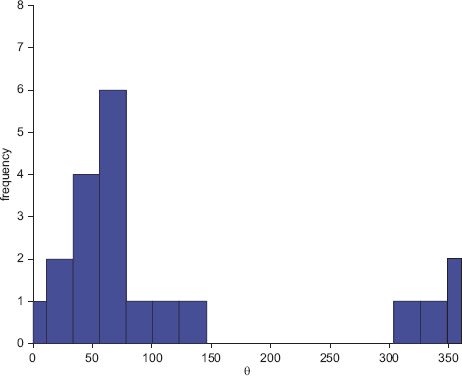
FIGURE 7.1 Histogram of angular data

Note that the estimate of the mean is identical to the sample circular mean, but there is no simple conversion between the circular variance and K. A normal or Gaussian distribution has a parameter representing the mean and the variance of the distribution, and in the case of the von Mises distribution there is a parameter for the mean, but the K parameter does not have a simple relationship with the circular variance. While 1 / K might reasonably be seen as analogous to the variance, 1 / K = 0.4364 is quite different from the computed circular variance, which is 1 – = 0.2588.

The probability density function (pdf) of the fitted von Mises distribution is shown in Figure 7.2.

It can be useful to draw a rose diagram, which is the circular analogue of a histogram, or a plot of the pdf on polar coordinates; these are given in Figures 7.3 and 7.4. The main advantage of the circular plot is that there is no arbitrary edge at 0 or 2π radians or at 0 or 360 degrees. The possible disadvantage is that intuition may be worse in a circular plot as they are less familiar, and it may be difficult to read the magnitude on a rotated axis.

The fact that the von Mises distribution has sufficient statistics makes it a very convenient form to analyse circular datasets. However, other distributions are also of interest.

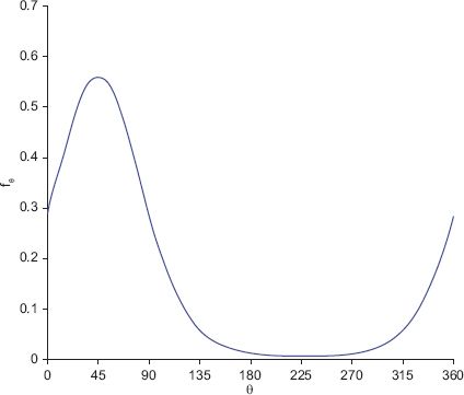
FIGURE 7.2 The pdf of a von Mises distribution fitted to the data shown in Figure 7.1

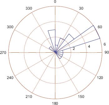
FIGURE 7.3 Rose diagram

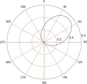
FIGURE 7.4 The pdf of a von Mises diagram fitted to the data shown in Figures 7.1 and 7.3

One way to construct a circular distribution from a distribution with real support G() is to use modular division (Ferrari, 2009); recall that taking modular division with 2π is equivalent to taking the remainder after dividing by 2πand then multiplying this number by 2π. Thus

The pdf can then be constructed with an infinite sum

where f_ω(ω) is the density of G().

The infinite sum is inconvenient, although it can be removed in special cases such as the wrapped Cauchy distribution. Unfortunately, it cannot be removed in the more interesting case of the wrapped normal distribution. The wrapped normal is of interest because it arises when applying the central limit theorem on the circle; also, the convenient properties of the multivariate normal are useful in multivariate statistics and the wrapped normal also enjoys other convenient mathematical properties: e.g. the sum of two independent wrapped normal distributions is also wrapped normal. While for linear statistics the normal distribution has a variety of convenient analytical properties, for circular statistics these convenient properties are awkwardly shared between the von Mises and the wrapped normal distributions.

The absence of sufficient statistics requires the use of numerical methods such as the expectation–maximisation (EM) algorithm in order to fit wrapped distributions; the rather technical details are given in Fisher and Lee (1994) with more background given in Jammalamadaka and Sengupta (2001), and a Markov chain Monte Carlo approach is outlined for fully Bayesian inference in Ravindran (2003) and Ferrari (2009). Fortunately, modern software libraries, particularly those provided in the R circular package, mean that implementing these complicated algorithms is usually unnecessary for the practitioner. A fit applied to the same data gives μ = 0.2549π or 45.3 degrees and σ = 0.5162, and a circular plot of the pdf is shown in Figure 7.5, which shows it to be a very similar shape to the von Mises. For completeness a wrapped Cauchy is shown in Figure 7.6 which also has a very similar shape, but is a little more concentrated and as a result the mean is slightly shifted.

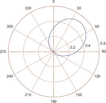
FIGURE 7.5 The pdf of a wrapped normal fitted to the dataset shown in Figure 7.1

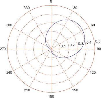
FIGURE 7.6 The pdf of a wrapped Cauchy fitted to the dataset in Figure 7.1

Semi-parametric and non-parametric methods

So far we have seen how circular data can be summarised by descriptive statistics that correspond to the sufficient statistics of the von Mises distribution, and we have also shown how the von Mises distribution can be fitted to data as well as the wrapped Cauchy and wrapped normal distributions. A general limitation of these models is that they are relatively simple; nevertheless these simple distributions are useful in order to produce more complex semi-parametric and non-parametric statistical methods.

Mixture models as semi-parametric models

An effective way to construct a more complex distribution, is by the use of a mixture model with K components which has the following pdf m_θ(θ) and is constructed from a number of individual components f_θ(θ)

Efficient algorithms exist for the estimation of such models, including the widely used EM algorithm.

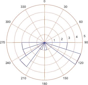
FIGURE 7.7 Rose diagram of a multimodal dataset

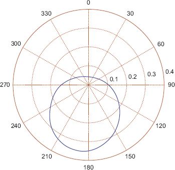
FIGURE 7.8 The pdf of a von Mises distribution fitted to the dataset in Figure 7.7

In order to consider why it might be necessary or desirable to use a mixture model, consider the dataset displayed in Figure 7.7. It is fairly easy to see that all of the methods we have considered so far will fail in one way or another. The average angle is –0.0184π or –3.3187 degrees, which is nowhere near the main modes observed at 50 degrees and 240 degrees. The variance for the data is quite large at 0.8645 (recall that the maximum value is 1), which, assuming a von Mises distribution, suggests that the data is near uniform instead of the two distinct modes observed. A polar plot of the pdf of the von Mises distribution is shown in Figure 7.8. In contrast, when a mixture of two von Mises distributions is fitted to the data, the two modes are located at 51.1 degrees and 246.6 degrees; a plot of the pdf of the mixture model is shown in Figure 7.9.

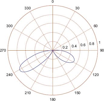
FIGURE 7.9 The pdf of a mixture of two von Mises distributions fitted to the dataset in Figure 7.7

There are some possible difficulties with this methodology. The first is that the number of mixture components K must be selected. While it seems straightforward in the given case study that K = 2 is preferred, this is not always clear for real datasets. Moreover there is no easy statistical solution to this type of problem, and traditionally heuristics are employed such as the use of cross-validation or human intuition to select K. The EM algorithm also occasionally shows numerical problems failing to converge to the optimal solution or, in rare cases, finding a singularity in the likelihood. Failure to converge can usually be mitigated by rerunning the algorithm, while singularities can be avoided by preventing k becoming too large and thereby preventing one of the mixture components being a sharp spike of probability mass centred on a single data point.

The technical details of the EM algorithm for the Fisher–von Mises distribution are given in Banerjee et al. (2005); again, fortunately, libraries such as Hornik and Grün (2014) in R or the simple MATLAB implementation included in the code accompanying this chapter reduce the need for practitioners to be overly concerned with implementation details.

Kernel smoothing as a non-parametric method

An alternative and very flexible approach to estimating a pdf is to use kernel density estimation, also known as Parzen’s window (Hastie et al., 2005), which amounts to using the following expression as an estimate of the predictive distribution:

Here is the kernel being used, and for circular problems, this is often set to be the von Mises distribution, which makes sure the estimated distribution has correct support and correctly handles the change-point problem at 0 or 2π. The bandwidth, given by , is an important free parameter that must be set carefully, although no generic solution is known, and again, heuristics such as cross-validation or human judgement must be employed.

A demonstration of the technique using the dataset from Figure 7.7 and a von Mises kernel with k = 20 and k = 100 is presented in Figures 7.10 and 7.11, respectively. When k is smaller and consequently the bandwidth is larger, a much smoother estimate results, as is shown in Figure 7.10; and when k is larger and the bandwidth is smaller, a more delicate estimate results, more vulnerable to noise, as in Figure 7.11.

Testing

Testing is a vexed subject in statistics, and perhaps no topic more so than the use of p-values. In a relatively positive paper on the subject, Senn (2001) recommends not relying on p-values alone, using likelihood as well as well as reporting point estimates and standard errors, and considering the use of Bayesian methods (amongst other things!).

With these qualifications noted, here we introduce a circular analogue for testing whether two quantities are independent. A test of this form involves the computation of a statistic T(x), a function of the two datasets that returns a real number; furthermore, we need to know what the distribution of T under the null hypothesis is. The statistic T(x) is computed on the real data, and then the probability of the statistic, or a more extreme value, is computed as the p-value. If the p-value is suitably low, then it is reasonable to say that either the null hypothesis is wrong or something unusual happened. The peculiarities of circular statistics enter when finding a reasonable definition of the statistic T(x). In cases where the data consist of real numbers a simple statistic such as the difference in means might suffice, but, as noted, computing differences with circular quantities constitute a problem.

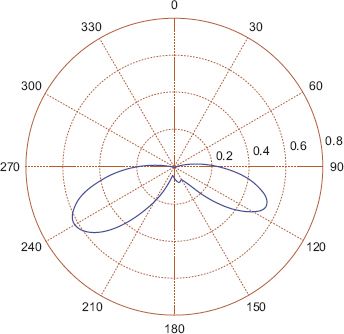
FIGURE 7.10 Kernel density estimate of pdf using the data shown in Figure 7.7 with a von Mises kernel with κ = 20

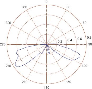
FIGURE 7.11 Kernel density estimate of pdf using the data shown in Figure 7.7 with a von Mises kernel with κ = 100

In order to give an example, a bivariate problem will be considered where the first example dataset θ¹ will be used. As noted earlier, this details the direction of a passenger travelling on the bus network, and the second datset θ²will be considered, which relates to the direction of travel for the journey to work for the same passenger. A question of interest might be whether the model should utilise the joint distribution or whether an independence assumption can reasonably be made by implying .

In order to make this approach as flexible as possible, Brunsdon and Corcoran (2006) propose as a statistic the mutual information between the two densities, estimated using the above kernel smoothing approach. This results in the statistic

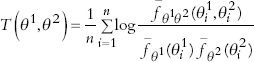
where θ¹ refers to the first sample which has estimated density refers to the second sample which has estimated density , the estimated joint density is and the number of data points is n. If the two distributions are independent then the mutual information is 0.

As this is a complicated statistic, there is no known form for the sampling distribution, and instead computational methods such as drawing random permutations of mismatching θ_i¹, θ_i² (i ≠ j) can be used in order to sample from the statistic conditional on the null hypothesis, or alternatively the very general bootstrap procedures proposed by Efron and Tibshirani (1993) can also be adopted, as it is here. This methodology, as stated, is quite a generic method for carrying out a test of independence of two distributions; the adaption to circular statistics occurs by using a von Mises kernel in order to carry out the density estimation.

In order to demonstrate this method, the test is applied to the two presented datasets using k = 20. A colour map representing the joint pdf of the joint estimate is shown in Figure 7.12(a), and one representing the product of the two densities separately estimated is shown in Figure 7.12(b); the similarity suggests that the two distributions might be close to being independent.

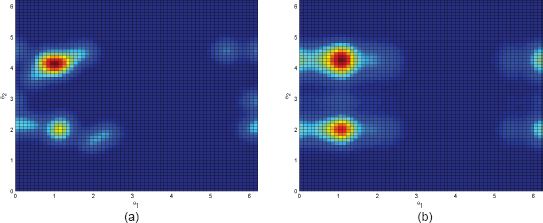
FIGURE 7.12 (a) The joint estimate of . (B) The product of the marginal estimates

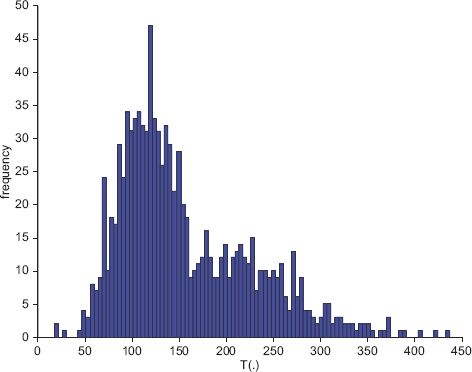
FIGURE 7.13 Bootstrap simulations of the sampling distribution

The statistic takes the value T = 113.8; when we bootstrap samples from the distribution of the statistic we find that the probability of this value being more extreme (i.e. of greater value) is 0.666, which indicates that the null hypothesis of independence is not rejected. This finding is consistent with the observation that the two estimates in Figure 7.12 are quite similar. Also note that the value 113.8 is a fairly typical mid-range value in the sampling distribution (see Figure 7.13: the higher the value, the less compatible the statistic is with independence).

While the test found that the data were consistent with the hypothesis that the two datasets are independent, in practical situations there are often compelling a priori reasons to believe that there will be some sort of dependence between distributions, and in a situation like these, with fairly small sample sizes, the failure to find a difference between the joint distribution and the product of the marginal may be because the dataset is too small to detect such differences. Users of these tests should bear in mind the impact of effect size and sample size on the outcome of the test. Testing within the context of circular data is a large well-studied topic and much more information about circular statistical testing can be found in Mardia and Jupp (2000).

A case study modelling direction of travel of bus commuters

Brisbane, Australia’s third largest city and Queensland’s state capital, has a relatively extensive bus network which includes over 400 bus routes and 10,000 bus stops. The origin and destination of hundreds of thousands of trips per day can be tracked by means of electronic ticketing or smart cards. An important problem from a transport planning perspective is to determine the volume of people travelling between given origins and destinations and how this varies from location to location.

A simplified extract from the 150,000 record smart card dataset is shown in Table 7.1, which for the purposes of this study includes information capturing the location (in (x, y) coordinates) of each trip origin and destination, or, in other words, the bus stop at which the passenger began and completed their journey.

In order to conduct the circular analysis of Brisbane, the city is divided into a 14 by 14 grid, and for each cell in the grid, the set of trips that originate from that cell are aggregated for analysis. The amount of data available per cell is variable and in some cases away from the bus network the cells are empty.

TABLE 7.1 Smart card dataset

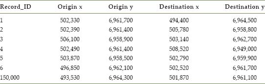
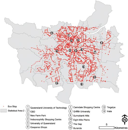
FIGURE 7.14 Case study region

First, a simple method to model the data is to compute the circular mean for each of these locations, the results of which are shown in Figure 7.15. Perhaps unsurprisingly, the main direction of travel from almost the entire area of the city is towards the central business district (CBD, number 2 on the map). While the circular mean is obviously identifying the strongest trend, it is neglecting to detect when passengers move from a non-central location to some other non-central location. It seems reasonable to suppose that the circular distributions obtained at a number of locations around the city will have multiple modes, indicating multiple important lines of direction. This can be confirmed by plotting rose diagrams, or alternatively by using kernel density estimation for some of the locations. Consider the location highlighted in Figure 7.16 which is on the outskirts of the city in the South West; a rose diagram for the angular data is shown in Figure 7.17, a graphical representation of the mean angle in Figure 7.18 and a kernel density estimate in Figure 7.19. From these plots it is confirmed that there are several directions of flows of differing importance from passengers in this region, and summarising this with the mean direction of flow shown in Figure 7.18 is unsatisfactory. A much better fit is given by a four-component mixture of von Mises distributions, with the pdf of such a fit shown in Figure 7.20, and a plot of the direction and strength of the four modes shown in Figure 7.21. The significance of Figure 7.21 is that the four preferred directions of flow can be summarised by four circular parameters representing the means of the four components of the mixture model. The choice of four mixture components makes intuitive sense in this case as the rose diagram shows four clear modes, but in other regions it may make sense to have fewer or more modes.

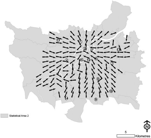
FIGURE 7.15 Mean directions of travel for bus passengers in Brisbane

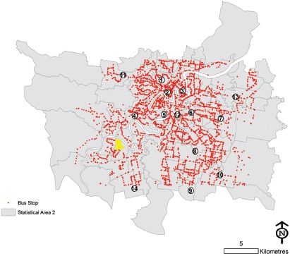
FIGURE 7.16 Selected region (in yellow) for detailed analysis of directions of travel

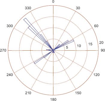
FIGURE 7.17 Rose diagram of the direction of travel on the selected data in Figure 7.16

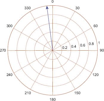
FIGURE 7.18 Given the multimodality of the distribution, the circular mean is a poor summary of the direction of travel on the selected data in Figure 7.16

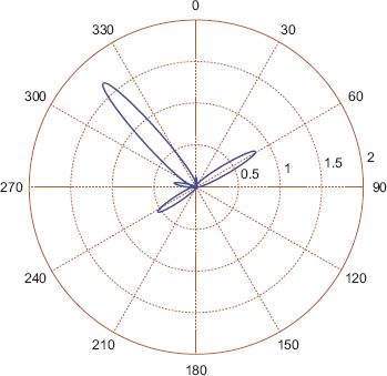
FIGURE 7.19 Kernel density estimate on the selected data in Figure 7.16 with κ = 100

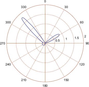
FIGURE 7.20 The pdf of the estimated four-component mixture of von Mises model estimated on the selected data in Figure 7.16

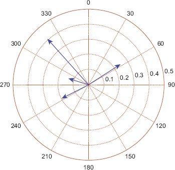
FIGURE 7.21 The four modes found using a four-component mixture of von Mises model on the selected data in Figure 7.16

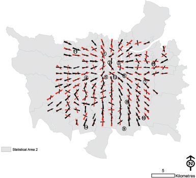
FIGURE 7.22 The direction and strength of travel on a 14 by 14 lattice estimated using a two-component mixture model

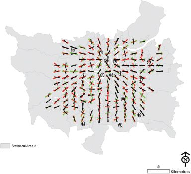
FIGURE 7.23 The direction and strength of travel on a 14 by 14 lattice estimated using a three-component mixture model

In order to build up a picture of secondary flows around a city, a two-component mixture model was fitted to the same dataset, and the two arrows plotted in Figure 7.19. A similar procedure was followed using a three-component mixture model in Figure 7.20 and a four-component one in Figure 7.21. The advantages of using the mixture model approach are immediately apparent as it is now possible to identify corridors of movement that are not moving towards the centre of the city but rather run across it. Without the semi-parametric mixture model approach only the most obvious city-bound trips could be extracted. The question of how many components should be used in the mixture model is perhaps more vexed; interesting details become apparent as the number of components is increased, but also in many places only one or two components seem adequate. Ideally the number of components could be varied depending on the data and the particular location. Another issue of concern is that the EM algorithm is a local optimiser that usually does not find global solutions to the maximum likelihood problem; slightly different results will therefore be obtained due to different initial conditions on subsequent runs of the algorithm. The use of mixture models allows Figure 7.15 to be improved by plotting secondary directions of travel using two mixture model components as in Figure 7.22, or three mixture components as in Figure 7.23. This methodology appears useful in highlighting secondary corridors of travel flows to other significant locations distinct from the CBD.

Conclusions

Geographers deal with a wide range of different data types, and while there are many well-developed tools for real, count and categorical data based upon distributions with appropriate support, angular or circular quantities which are also of great interest to geographers receive considerably less attention. This chapter has addressed how circular statistics can be used for both descriptive and modelling analyses with the potential to offer new insights into spatial datasets and extend the geocomputational toolbox.

The most basic but useful idea presented is that the circular mean is a convenient way of summarising simple unimodal angular or circular datasets. The critical idea here is to convert the angles to a vector quantity on the unit circle, before computing the average and then converting the output back to polar coordinates. It was demonstrated that this simple idea mitigates the change-point problem, i.e. the closeness of points around [0, 2π] or [0, 360].Another simple statistic based upon the magnitude of this vector quantity that was shown to be a useful analogue of linear variance was referred to as circular variance.

In order to consider more sophisticated statistical methods it was necessary to introduce some distributions with support for angular or circular quantities. The easiest of these to use in practice is the von Mises distribution which has the mean computed on the rectangular representation of the angle, as used previously for descriptive statistics. The other common and useful way to use distributions with real support (i.e. the distribution applies to regular numbers including fractions and negative numbers) is to convert the model to one with the more limited support used for angles by wrapping the distribution around the interval [0, 2π] or [0, 360], thus giving the wrapped normal and wrapped Cauchy distributions amongst others. Both of these distributions can be fitted to datasets and therefore used for relatively simple univariate models. More complex modelling can be achieved using semi-parametric methods such as a mixture of von Mises distributions or non-parametric methods using kernel smoothing methods.

A case study of electronic smart card data was used in order to identify the main routes of travel in Brisbane, Australia. A simple analysis based upon applying circular means to a lattice of data found that the main directions of travel are predominantly towards the CBD. In order to further investigate the data, a particular region in the lattice was shown to contain multimodal structure that required either non-parametric or semi-parametric approaches. The mixture model approach was demonstrated to be particularly useful in identifying corridors of movement as each mixture component could be plotted as an individual arrow showing a general direction of movement. This allowed the identification of more subtle movements within the city.

In summary, the frequencies with which geographers might consider the analysis of direction suggest that there are many opportunities to employ a circular statistical and graphical approach to a wide variety of spatial datasets. It is hoped that this chapter highlights and promotes the ways in which circular statistics might be more routinely embedded within geographical analyses.

FURTHER READING

This chapter outlines the fundamental differences with analysing and modelling circular data, offers some techniques and demonstrates their usefulness with a case study. There has, however, been a great deal more development in this area. In this section we point the reader to some of the literature on more advanced topics of interest for the examination of geographical problems.

ACKNOWLEDGEMENTS

We would like to thank Translink for access to the data on which this chapter is based. However, the interpretations of the analysis are solely those of the authors and do not necessarily reflect the views and opinions of Translink or any of their employees.

Fisher, N.I. (1995) Statistical Analysis of Circular Data. Cambridge: Cambridge University Press.

A generic tool that has proven to be of great utility to geographers is the use of correlation or covariance to measure the relationship between two real variables, such as the determination of a relationship between income and level of education across a region. The use of correlation is complicated when one or more of the variables is an angular quantity. In order to deal with these issues useful empirical measures of correlation between two circular quantities or between a circular quantity and a linear quantity have been proposed in this text. Taking our earlier questions based on the commuting example, one could now explore whether the mean direction of commuter travel is correlated with the distance travelled across a region.

Lee, A. (2010) Circular data. Wiley Interdiciplinary Reviews: Computational Statistics, 2: 477–486.

A second topic of interest is that of regression modelling where the dependent variable is either a count or a real number. Again modifications are needed if the variable represents a circular or angular quantity. Common to the application of correlation and covariance, regression modelling has formed a core analytical backbone of a plethora of geographical studies. However, in its standard form it is not capable of integrating angular quantities. Circular regression methods (see the above text for a good entry point to this literature) offer the possibility to extend the conventional regression framework, permitting the investigation of new questions. Drawing on our commuting example, one could examine how the mean directions of travel across a region (as the dependent) are explained by a set of socio-economic variables such as age, income and industry sector of employment.

Jona-Lasinio, G., Gelfand, A. and Jona-Lasinio, M. (2012) Spatial analysis of wave direction data using wrapped Gaussian processes. Annals of Applied Statistics, 6: 1478–1498.

A final area of interest to geographers is the inclusion of a notion of spatial smoothing into the model. Geographers regularly employ models for real-valued data that incorporate space such as geographically weighted regression or the spatial autocorrelation model, all of which rely on the properties of the multivariate normal distribution. An adaption to circular or angular quantities requires a similarly useful probabilistic model. While there has been little work on multivariate circular distributions, the development of the wrapped Gaussian process outlined above is a notable exception that explicitly takes into account spatial aspects of the model, and Jona-Lasinio et al. (2012) demonstrate its ability in modelling wave direction.