Geocomputation: A Practical Primer (2015)

PART III

MAKING GEOGRAPHICAL DECISIONS

8

GEODEMOGRAPHIC ANALYSIS

Alexandros Alexiou and Alex Singleton

Introduction

Geodemographic classification has been defined as ‘the analysis of people by where they live’ (Sleight, 1997: 16); it involves categorical summary measures that aim to capture the multidimensional characteristics of both built and socio-economic characteristics of small geographical areas. This chapter outlines the origins of geodemographic classifications, how they are typically constructed, and their application through an illustrative case study of Liverpool, UK.

Within sociology and geography there is a legacy of identifying aggregate socio-spatial patterns within urban areas through a variety of empirical methods. From the early 1900s onwards, researchers tried to systematically document spatial segregation and establish a series of general principles about the internal spatial and social structure of cities, commonly motivated by the ill effects of residential segregation of the poor and ethnic minorities (van Kempen, 2002). Within the UK, Charles Booth’s poverty maps were one of the first attempts to map the socio-spatial structure of London in the early 1900s, although it was not until the late 1920s that the Chicago School formulated a comprehensive model of urban ecology, such as the concentric zone model of Burgess and Park (Burgess, 1925). Their research was largely based on the then recently introduced census data, alongside extensive fieldwork and map-making (Burgess, 1964: 11–13).

The analysis of detailed demographic, social and economic census data was further developed through the work of Shevky and Bell (1955). Their work introduced ‘social area analysis’, a methodology focused on a three-factor hypothesis that aimed to assert a typology of urban places measured in terms of urbanisation, segregation and ‘social rank’ (Brindley and Raine, 1979). This analytic framework inspired the adoption of a set of tools and techniques encapsulating a broader range of socio-economic census variables (Tryon, 1955; Rees, 1972), and such theoretical approaches were later collectively known as ‘factorial ecologies’, due to a widening of those aspects used to explain urban structure (Janson, 1980). Factor analysis (and, similarly, principal component analysis) dominated such quantitative geography in the 1970s, and was largely used to identify major underlying attributes of spatial structure, albeit with debatable results. Factorial studies were criticised not only because of their lack of theoretical context (Berry and Kasarda, 1977), but also because of their methodological weaknesses, for example their lack of extendability that constrained them to being city-specific (Batey and Brown, 1995).

During this period, much scholarly concern was also focused on the interpretation and categorisation of the fundamental processes by which cities operate. In spite of the numerous attempts to classify cities per se, studies failed to find a unified theory of city typology – if such a functional typology ever existed. Classifications started to focus alternatively on smaller-area geography, and on the ‘methods flowing from identification of variations of cities and following from the selection of dimensions relevant to a specific purpose’ (Berry, 1972: 2). There was a common belief that typologies aid in generalisation and prediction, and urban classification was much more comprehensive when applied with a narrow scope, in terms of both area and purpose.

Within such context, geodemographics emerged in both the United States and United Kingdom during the late 1970s as an extension of these earlier empirically driven models of urban socio-spatial structure. Geodemographic classifications organise areas, typically referred to as neighbourhoods, into categories or clusters that share similarities across multiple socio-economic and built environment attributes (Singleton and Longley, 2009).

Despite a lineage of use, geodemographic classifications lack a solid theory. In nomothetic terms, many view geodemographics as methodologically unsatisfactory since the underlying theory can be considered as ‘simplistic’ and ‘ambiguous’ (Harris et al., 2005). The conceptual framework is based on a fundamental notion in social structures, homophily – the principle that people tend to be similar to their friends. This manifests spatially as a general tendency for people live in places with similar people, much like the ‘birds of a feather flock together’ adage suggests; and it is consistent with Tobler’s first law of geography, that ‘everything is related to everything else, but near things are more related than distant things’ (Tobler, 1970: 236). However, one paradox is that despite geodemographic representations showing spatial autocorrelation between taxonomic groups, the methods for building geodemographics as currently construed can be considered contradictory to Tobler’s statement. The aggregations of zones into categorical measures based on attributes sweeps away contextual differences between proximal zones; and as such, the final classifications assume that areas within the same cluster have the same underlying characteristics. Standard geodemographic techniques have failed to incorporate near geography in a sophisticated way, and despite the term, geodemographics are in fact aspatial. Thus far, there have been very few attempts to build a unified framework, at least within which the relative benefits of both spatial interaction and geodemographic approaches can be maximised (see, for example, Singleton et al., 2010). For many applications, the issue of geographic sensitivity is usually experienced when normalising input variables globally and without taking into account local variation extents, thus obscuring potentially interesting local patterns. For instance, some argue that the relationship between areal typology and behaviour might not be spatially constant (Twigg et al., 2000). This type of ecological fallacy raises a series of methodological questions regarding the success of geoclassifications, given the high within-cluster variation that is already smoothed away (Voas and Williamson, 2001).

Geodemographic classification systems

Geodemographic analysis was initially developed as a ‘strategy’ that can be used to identify patterns from multidimensional census data (Webber, 1978). However, current geodemographics may use a variety of public and private data to generate profiles (Birkin, 1995). Some of the pioneering studies were applied in the UK to identify neighbourhoods suffering from deprivation (Webber, 1975). However, in the USA, geodemographics were first utilised in the private sector, as the macro-economic conditions, alongside the freedom-of-information tradition, created an environment that quickly enabled the exploitation of census data commercially (Flowerdew and Goldstein, 1989), and the first commercial applications started appearing during the early 1980s. In the following years, geodemographic classifications gained large popularity as their utility was demonstrated across a variety of applications – from strategic marketing and retail analysis to public sector planning (Birkin, 1995; Brown et al., 2000).

Despite a common starting point, there are arguably critical differences between the UK and the USA, as geodemographics evolved through different paths. While the US classifications have typically been commercial, in the UK context there is a long history of free and more recently open classifications, and they have seen greater application in public policy and academia (for a detailed review, see Singleton and Spielman, 2014). More generally, in the UK there has been a recent renaissance of interest in geodemographics from the public sector, mainly driven by government pressure to demonstrate value for money and the advent of new application areas (Longley, 2005).

For instance, Batey and Brown (2007) developed a method of evaluating the success of area-based initiatives by using a geodemographic classification to produce spatially targeted socio-economic profiles. In this way, they assessed the efficiency of spatially targeted urban policies by examining how many of the people these contained are in fact not those for whom the initiative is intended, in which case it is defined as inefficient or incomplete. Singleton (2010) and Singleton et al. (2010) explored patterns of access to higher education by linking summary measures of local neighbourhood characteristics with individual-level educational data; and through a spatial interaction framework, demonstrated the size of spatial flows between socio-economically stratified areas and institutions, with the aim that such a tool could be used by key stakeholders to examine potential policy scenarios.

Geodemographics have also been recently used in health screening epidemiology, where detailed geographical information is often unavailable. In these studies, finer geographic granularity is necessary in order to produce targeted ecological estimates and infer interaction effects between health and demographics (Aveyard et al., 2002). Small-area aggregates can also be used to increase statistical power, as small-area ecological data can alleviate bias due to measurement errors in individual-level data (Jackson et al., 2006). Other notable examples include the application of geodemographics in policing (Ashby and Longley, 2005). Geodemographic analyses of local policing environments, crime profiles and police performance can provide a neighbourhood classification that is produced explicitly to reflect differing policing environments and help allocate policing resources accordingly.

The composition of geodemographic classification differs quite radically depending on the scope and probable usage by the intended stakeholders; as a result, available geodemographic products include a variety of classification systems. Among the conventional general purpose classification systems are some privately developed classifications such as Mosaic (Experian), Acorn (CACI), P2 People and Places (Beacon Dodsworth), MyBestSegments (Nielsen) and CAMEO (EuroDirect). Such commercial geodemographic systems produce discrete classes primarily designed to describe consumption patterns. As such, their respective databases are not only populated with census data but compiled from large sets of consumer dynamics such as credit checking histories, product registrations and private surveys (Singleton and Spielman, 2014). Open classifications, on the other hand, are those that can be accessed by the public without cost, have transparent published methodologies and comprise freely available input data. One of the most popular open classifications available in the UK is the Output Area Classification (OAC) provided by the Office of National Statistics (see Vickers and Rees, 2007).

Building a geodemographic classification

Building a successful classification may seem fairly straightforward but it can be a difficult and very time-consuming process. It is important that a classification addresses end-user needs, but is also impacted by data availability, coverage and potential weighting (Webber, 1977). Harris et al. (2005) provide a good basis for the methodologies typically used to build geodemographic classifications, and also provide some examples in the UK context. Vickers and Rees (2007) also provide a detailed step-by-step analysis of the process of creating the OAC geodemographic classification, which was built upon previous work on clustering methodologies by Milligan (1996) and Everitt et al. (2001). Less is known about how geodemographic classifications are built within the private sector, beyond those details usefully presented in Harris et al. (2005). Commercial geodemographic classifications have an inherent commercial confidentiality, and as such, most of their methodologies remain a ‘black box’, which some have argued impairs not only reproduction, but also scientific questioning of the ways in which the clusters emerged from the underlying data(Longley, 2007; Singleton and Longley, 2009).

Scale, variable selection and evaluation

The first stage in building a geodemographic classification is to assemble a database of inputs that are deemed important for differentiating areas. The geographical unit of reference used to collate such data will depend on the purposes of the classification, and also pragmatically on those data available to the classification builder at different scales (including licensing constraints). For example, most open (and some commercial) geodemographic systems in the UK are based on data aggregated at the Output Area level, where zones represent an average population of approximately 300 people, and is the smallest scale at which public census data are provided. However, different sets of variables can have different scales and there are various ways in which these are managed, ranging from simple apportionment from aggregate to disaggregate scales, small-area estimation or microsimulation (Birkin and Clarke, 2012).

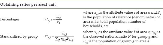
From the outset, geodemographic methods have typically employed a pragmatic variable selection strategy, combining the experience of the classification builder (what is deemed to work) with the overarching purpose of a classification (what is required), alongside some degree of empirical evaluation. Attributes can be collected and compiled with a variety of measurement types including percentages, index scores, ratios or composite measures (e.g. principal components). When standardising values it is important to remember that sometimes variables have varying propensities among different groups of people, typically by age or sex (Table 8.1). For instance, long-term illness indices frequently have higher values between groups of older people. An area that has a higher ratio of older to younger people will, ceteris paribus, tend to have higher rates of illnesses as well. In these cases, age standardisation is recommended since it can scale values in accordance with age structure; scaled ratios are calculated as the sum of the age-specific rates multiplied by the area population per age group. If area specific rates are not provided, they could be obtained from the national or regional average.

TABLE 8.1 Data formatting per aerial unit

When managing quantitative data, in many cases variables will not seem appropriate to use in their raw format. Available data can have skewed distributions, contain a high rate of missing values or originate from sample sizes smaller than desired, thus generating uncertainty. In general, a detailed assessment of each variable is typical prior to the clustering process in order to identify ‘unfit’ data. Evaluation typically includes mapping, distribution plots (such as histograms) and correlation analysis.

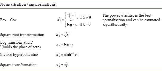
A particular issue for effective cluster formation is non-normality of attributes or skew. Common techniques used to address this issue include normalisation of the variables when applicable, or weighting to adjust their influence on the final classification when normalisation is deemed by the classification builder not to be appropriate. Normalisation is the process of transforming the variable values to approximate normal distributions, usually through various power transformations. Other treatments include weighting or using principal component analysis to identify common vectors of variables that help reduce data complexity and noise (Harris et al., 2005). Table 8.2summarises those common transformations used in geodemographics.

TABLE 8.2 Variable transformations used for normalisation

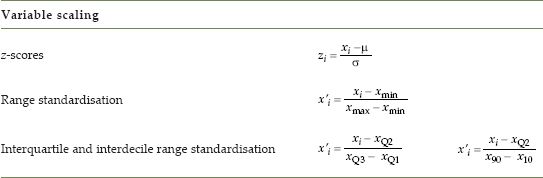
Finally, a universal scale of measurement should be applied to every observation prior to clustering, such as range standardisation or standardised z-scores (Table 8.3), given that disproportionate measurements will frequently affect the dissimilarity function of the clustering technique towards variables with higher values. Techniques such as interquartile and interdecile range standardisation are useful when data contain outliers.

TABLE 8.3 Variable transformations used for scaling

Clustering approaches and techniques

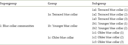
Clustering approaches and techniques can differ quite radically, depending not only on the purpose, but also on the nature of the data to be clustered (for a more in-depth analysis of clustering techniques, see Everitt et al., 2001; Hastie et al., 2009). A geodemographic typology is usually presented as a hierarchy; with different clusters produced for varying tiers of aggregated areas (Table 8.4). Such a hierarchy can be created from the top or the bottom. A top-down approach includes the creation of larger groups of cases that are subsequently divided into smaller subgroups. This method is typically implemented with the K-means clustering algorithm, and was used to produce the 2001 OAC, which included seven supergroups, which were respectively split into 21 groups and further into 52 subgroups.

TABLE 8.4 an example of a nested hierarchy for the ‘blue collar communities’ supergroup cluster from the 2001 Output Area Classification

A bottom-up approach is, however, more prevalent within the commercial sector, and includes the creation of numerous smaller groups (using K-means), which are then aggregated based on their similarities into larger groups (typically with hierarchical algorithms such as Ward’s clustering).

K-means clustering uses squared Euclidean distance as a dissimilarity function, and so can be used only when variables are of a continuous measurement type. Essentially, K-means clustering assigns N observations into K clusters in such a way that, within each cluster, the average distance of the variable values from the cluster mean is minimised. Taking into account that for any set of observations S there is an argument that describes the minimum squared distance defined as

then for the aggregate of the total clusters there is a set of arguments that minimise the total within cluster variation of the multidimensional data points:

where WCSS is the within-cluster sum of squares for a cluster distribution C with K seeds, is the data observations and is the k-cluster mean.

K-means is typically initiated with a random set of initial seeds, and then the algorithm assigns every observation to a seed based on the least squared distance. New means based on the assignments and then calculated, and observations reassigned to their new nearest cluster mean, again based on the least squared distances. The algorithm ‘converges’ when the within-cluster sum of squares is minimised, i.e. when the cluster assignments no longer change. This technique is straightforward to implement and perhaps explains the popularity in the classification of multidimensional inputs; however, the K-means algorithm needs a specific predetermined number of clusters (K), and furthermore, results can differ based on the initial k centres that are selected. As such, it is typical to run K-means multiple times for an analysis, extracting the results for each converged cluster set, and evaluating them on the basis of some metric – most commonly, an effort to minimise the within sum of squares (i.e. more compact, and therefore homogeneous clusters).

In hierarchical cluster analysis, Ward’s algorithm can be applied to merge clusters with the least amount of between-cluster variance, thus producing the minimum increase in total within-cluster variance after merging (Everitt et al., 2001). Ward’s clustering criterion is typically used in those geodemographics created from the bottom up to produce the more aggregate hierarchy of clustering typologies.

Although more prevalent in research rather than commercial applications, there are multiple other clustering techniques that have been implemented within the context of area classification. A self-organising map (SOM) is an unsupervised classifier that uses a type of artificial neural network to classify space (see Spielman and Folch, Chapter 9), based on the configuration of attributes that ‘fit’ each neuron (Skupin and Hagelman, 2005). Typically the SOM mapping process employs a lattice of squares or hexagons as the output layer, and the results are therefore easily mapped. SOMs have been tested as an alternative classifier of census data in the UK (Openshaw and Wymer, 1995) and the USA (Spielman and Thil, 2008) where they seem to perform well for socio-economic data at the census tract scale. They also have the advantage of not assuming any hypotheses regarding the nature or distribution of the data, and respond well to geographic sensitivity.

Another methodology to classify areal units is based on fuzzy logic algorithms or ‘soft’ classifiers. Fuzzy classifications have the inherent ability to assign spatial units to more than one cluster with varying membership values (i.e. probabilities). The degree of membership reflects the similarities or dissimilarities between groups and therefore is often addressed as a soft classifier (in contrast to hard classifiers such as K-means). Most studies regarding geodemographic analysis that use fuzzy classification employ the Fuzzy C-means algorithm or the Gustafson–Kessel algorithm (Feng and Flowerdew, 1998; Grekousis and Hatzichristos, 2012).

Other probabilistic classifiers that have been used less prevalently are multinomial logistic regression models, also known as m-logit models. A logit model has the advantages of using continuous, binary or categorical data to generate clusters, and these can also be considered as a soft classifier as they output the probability of areas belonging to each cluster category. Such models have been used in health geodemographics and epidemiology, where detailed geographical information is often unavailable (Jackson et al., 2006).

Cluster analysis and interpretation

The final step in building a geodemographic classification includes the review and testing of the cluster results, alongside description of the typology. For example, checking the size of clusters is one of the basic steps in the optimisation procedure. Clusters with relatively low representation of cases should generally be avoided, by either adjusting the number of clusters or by the re-evaluation of the data input. Furthermore, if, measured in terms of variance, two or more of the output clusters may look very similar, and merging might be considered, and inversely split if the clusters are too large. Harris et al. (2005) provides a ‘rule of thumb’ for merging similar clusters, if the loss of variance within the dataset is less that 0.22%. Other ways to test an output classification is to correlate it with existing classification systems, or via sampling, such as cross-tabulation with geocoded survey data.

If the classification appears successful, a final stage is typically naming and describing the resulting clusters with written ‘pen portraits’ that best fit the profile of areas represented by the clusters. The process of creating such descriptions can be quite difficult, especially in lower hierarchies, where the cluster dissimilarities are more subtle (Vickers and Rees, 2007). Here is an extract of the profile for the ‘affluent achievers’ cluster from the Acorn commercial classification by CACI:

These are some of the most financially successful people in the UK. They live in wealthy, high status rural, semi-rural and suburban areas of the country. Middle aged or older people, the ‘baby-boomer’ generation, predominate with many empty nesters and wealthy retired. Some neighbourhoods contain large numbers of well-off families with school age children, particularly the more suburban locations. These people live in large houses, which are usually detached with four or more bedrooms. (CACI, 2013)

Classification systems also commonly augment such descriptions with other visual materials such as photographs, maps and bar graphs or radar charts. Depending on the intended end-users, labelling and description must be selected appropriately in order to expand the user’s understanding of the group, while taking into account that the end user might not be accustomed to geodemographic classifications.

Liverpool Case Study

In this final section, a practical example of creating a geodemographic classification will be presented. For this purpose, the Local Authority of Liverpool will define the extent of the classification, which includes 1584 Output Areas. The analysis uses the R statistical programming language, and the dataset is assembled in its entirety with 2011 census variables, provided by the Office for National Statistics and aggregated at the Output Area level.

Methodologically, the cluster analysis follows a similar approach to that of the 2001 OAC, although it only aims to capture broad socio-economic categories for illustrative purposes. This analysis utilises the K-means clustering algorithm and produces a single aggregate typological level. As a first step, consideration was required to identify those variables that would form useful inputs to the classification. Although the census includes a very wide variety of potential candidate variables, a large number of them are homogeneous across space or highly correlated. For variables to be effective in a classification they should ideally show variation over space. For instance, any variation by sex is considered to be of lower importance, since the majority of Output Areas have the same overall ratio of males to females. Furthermore, given the urban location of this case study area, variables that captured dichotomies between urban and rural space might also be considered as less useful for any resulting classification.

Three elements were initially selected to guide the classification process and included demographic, housing and economic activity indicators. In total, 29 preliminary attributes were selected over the three taxonomical elements (Table 8.5).

TABLE 8.5 Initial dataset used for the liverpool classification

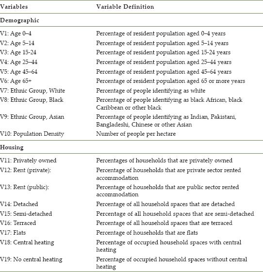
TABLE 8.5 (Continued)

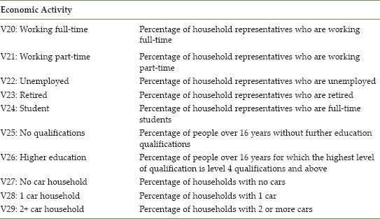
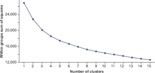
FIGURE 8.1 K-means: distance from mean by cluster frequency

The variables were each transformed into percentages, taking into account their respective denominator, with the exception of density, which was the only non-percentage variable. The next stage was to check how the variables were distributed and correlated, and assess for any that might negatively affect the clustering process. On the basis of variables with problematic distributions, these were removed from the initial dataset. Following the 2001 OAC methodology (Vickers and Rees, 2007), a log transformation was fitted to the variables to create more normal distributions. A cross-correlation table was then generated to show those variable pairs with high correlation, and a number of further attributes were selected for removal on this basis, thus aiming to reduce redundancy within the input data, and also limit bias towards any particular dimension being measured.

The variable selection process returned 17 variables that would form the input data to the K-means clustering, and were then scaled uniformly with z-scores. In order to address the question of how many clusters might be suitable, a within-cluster sum of squares distance graph (scree plot) was used to help identify a point at which the total distance only marginally improves the cluster homogeneity (also known as the elbow or knee criterion). However, in this case (Figure 8.1) there is no significant elbow visible, and as such, for these illustrative purposes we select K = 5 as a number of clusters that would be useful when mapping urban areas – increasing the classes would create a more detailed, but potentially less easily interpretable representation.

The K-means algorithm was subsequently run 10,000 times, and the result returning the least within-cluster total distance through these multiple iterations was extracted as the optimal result. The cluster sizes were then checked, and these varied between 72 and 522 output areas. This size variation is within acceptable limits, taking into account the limited extent of the analysis area. A useful way of obtaining information about how variables load onto each cluster is through a radar plot. Figure 8.2 shows a summary of the distribution of values within Cluster 2 (note that the Liverpool mean is 0). Cluster 2 consists mainly of neighbourhoods of middle-aged families, the majority of which are full-time workers with higher education degrees. Families are more prevalently living in low-density, detached houses, while the high ratio of car ownership indicates these areas may be more affluent. This cluster was named ‘white collar families’. A map of the other clusters and their attributed names can be seen in Figure 8.3. As discussed earlier, patterns exhibit a degree of spatial autocorrelation, despite locational proximity being absent from the classification.

FIGURE 8.2 Within-cluster variable analysis of Cluster 2

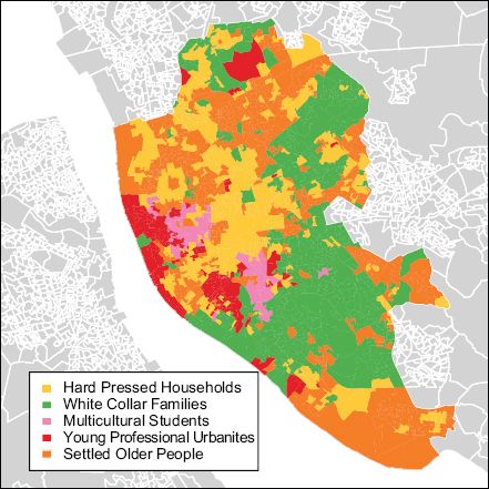
FIGURE 8.3 The final classification results, grouping the output areas of liverpool into five clusters

Conclusions

In the previous sections we have briefly outlined the history and application of geodemographic classifications, concluding the chapter with an overview of the basic process of building a geodemographic using a case study of Liverpool. While it is true that such applications can produce useful results, geodemographic research may face substantial challenges in the near future. Many geodemographics have historically relied on the analysis of the decennial census of the population, but institutional shifts in both the USA and UK are already changing the nature and availability of such data, given the growing costs associated with their collection (Singleton and Spielman, 2014). As such, the granularity currently offered by census data might not be readily available in the future; and as such, more research is needed into how the linkage of non-census attributes (both commercial and non-commercial) can be both validated and made more accessible for these purposes.

Secondly, geographic classifications, as currently construed, do not account for spatial relations between proximal zones. This traditional ‘aspatial’ approach has a number of implications when generating profiles. For marketing-related applications of geodemographics, a lack of local sensitivity may have fiscal implications, such as a reduced uptake of a product or service. However, in public sector uses, the consequences may be more severe, with mistargeting having potential implications on life chances, health and well-being. Hitherto, methods used to take into account near geography are typically geographically crude, accounting for spatial context through either an arbitrary zonal distance, or by division of areas into administrative units that may not correspond with the organisation of actual communities. Future research is needed to produce measures of near geography that can capture such associations and evaluate these vis-à-vis traditional geodemographic models.

FURTHER READING

For an excellent introduction to geodemographics, we would highly recommend Harris et al. (2005). More generally, the majority of research articles utilising geodemographic models can be found online at https://www.zotero.org/groups/geodemographics.