NoSQL for Mere Mortals (2015)
Part III: Document Databases
Chapter 8. Designing for Document Databases
“Making good decisions is a crucial skill at every level.”
—PETER DRUCKER
AUTHOR AND MANAGEMENT CONSULTANT
Topics Covered In This Chapter
Normalization, Denormalization, and the Search for Proper Balance
Planning for Mutable Documents
The Goldilocks Zone of Indexes
Modeling Common Relations
Case Study: Customer Manifests
Designers have many options when it comes to designing document databases. The flexible structure of JSON and XML documents is a key factor in this—flexibility. If a designer wants to embed lists within lists within a document, she can. If another designer wants to create separate collections to separate types of data, then he can. This freedom should not be construed to mean all data models are equally good—they are not.
The goal of this chapter is to help you understand ways of assessing document database models and choosing the best techniques for your needs.
Relational database designers can reference rules of normalization to help them assess data models. A typical relational data model is designed to avoid data anomalies when inserts, updates, or deletes are performed. For example, if a database maintained multiple copies of a customer’s current address, it is possible that one or more of those addresses are updated but others are not. In that case, which of the current databases is actually the current one?
In another case, if you do not store customer information separately from the customer’s orders, then all records of the customer could be deleted if all her orders are deleted. The rules for avoiding these anomalies are logical and easy to learn from example.
![]() Note
Note
Document database modelers depend more on heuristics, or rules of thumb, when designing databases. The rules are not formal, logical rules like normalization rules. You cannot, for example, tell by looking at a description of a document database model whether or not it will perform efficiently. You must consider how users will query the database, how much inserting will be done, and how often and in what ways documents will be updated.
In this chapter, you learn about normalization and denormalization and how it applies to document database modeling. You also learn about the impact of updating documents, especially when the size of documents changes. Indexes can significantly improve query response times, but this must be balanced against the extra time that is needed to update indexes when documents are inserted or updated. Several design patterns have emerged in the practice of document database design. These are introduced and discussed toward the end of the chapter.
This chapter concludes with a case study covering the use of a document database for tracking the contents of shipments made by the fictitious transportation company introduced in earlier chapters.
Normalization, Denormalization, and the Search for Proper Balance
Unless you have worked with relational databases, you probably would not guess that normalization has to do with eliminating redundancy. Redundant data is considered a bad, or at least undesirable, thing in the theory of relational database design. Redundant data is the root of anomalies, such as two current addresses when only one is allowed.
In theory, a data modeler will want to eliminate redundancy to minimize the chance of introducing anomalies. As Albert Einstein observed, “In theory, theory and practice are the same. In practice, they are not.” There are times where performance in relational databases is poor because of the normalized model. Consider the data model shown in Figure 8.1.
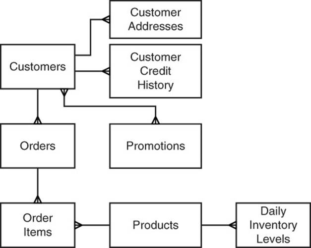
Figure 8.1 Normalized databases have separate tables for entities. Data about entities is isolated and redundant data is avoided.
Figure 8.1 depicts a simple normalized model of customers, orders, and products. Even this simple model requires eight tables to capture a basic set of data about the entities. These include the following:
• Customers table with fields such as name, customer ID, and so on
• Loyalty Program Members, with fields such as date joined, amount spent since joining, and customer ID
• Customer Addresses, with fields such as street, city, state, start date, end date, and customer ID
• Customer Credit Histories report with fields such as credit category, start date, end date, and customer ID
• Orders, with fields such as order ID, customer ID, ship date, and so on
• Order Items, with fields such as order ID, order item ID, product ID, quantity, cost, and so on
• Products, with fields such as product ID, product name, product description, and so on
• Daily Inventory Levels, with fields such as product ID, date, quantity available, and so on
• Promotions, with fields such as promotion ID, promotion description, start date, and so on
• Promotion to Customers, with fields such as promotion ID and customer ID
Each box in Figure 8.1 represents an entity in the data model. The lines between entities indicate the kind of relationship between the entities.
One-to-Many Relations
When a single line ends at an entity, then one of those rows participates in a single relation. When there are three branching lines ending at an entity, then there are one or more rows in that relationship. For example, the relation between Customer and Orders indicates that a customer can have one or more orders, but there is only one customer associated with each order.
This kind of relation is called a one-to-many relationship.
Many-to-Many Relations
Now consider the relation between Customers and Promotions. There are branching lines at both ends of the relationship. This indicates that customers can have many promotions associated with them. It also means that promotions can have many customers related to them. For example, a customer might receive promotions that are targeted to all customers in their geographic area as well as promotions targeted to the types of products the customer buys most frequently.
Similarly, a promotion will likely target many customers. The sales and marketing team might create promotions designed to improve the sale of headphones by targeting all customers who bought new phones or tablets in the past three months. The team might have a special offer on Bluetooth speakers for anyone who bought a laptop or desktop computer in the last year. Again, there will be many customers in this category (at least the sales team hopes so), so there will be many customers associated with this promotion.
These types of relations are known as many-to-many relationships.
The Need for Joins
Developers of applications using relational databases often have to work with data from multiple tables. Consider the Order Items and Products entities shown in Figure 8.2.
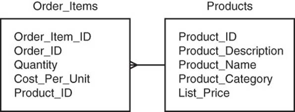
Figure 8.2 Products and Order Items are in a one-to-many relationship. To retrieve Product data about an Order item, they need to share an attribute that serves as a common reference. In this case, Product_ID is the shared attribute.
If you were designing a report that lists an order with all the items on the order, you would probably need to include attributes such as the name of the product, the cost per unit, and the quantity. The name of the product is in the Product table, and the other two attributes are in the Order Items table (see Figure 8.3).
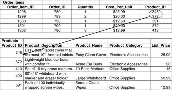
Figure 8.3 To be joined, tables must share a common value known as a foreign key.
![]() Note
Note
If you are familiar with the difference in logical and physical data models, you will notice a mix of terminology. Figures 8.1 and 8.2 depict logical models, and parts of these models are referred to as entities and attributes. If you were to write a report using the database, you would work with an implementation of the physical model.
For physical models, the terms tables and columns are used to refer to the same structures that are called entities and attributes in the logical data model. There are differences between entities and tables; for example, tables have locations on disks or in other data structures called table spaces. Entities do not have such properties.
For the purpose of this chapter, entities should be considered synonymous with tables and attributes should be considered synonymous with columns.
In relational databases, modelers often start with designs like the one you saw earlier in Figure 8.1. Normalized models such as this minimize redundant data and avoid the potential for data anomalies. Document database designers, however, often try to store related data together in the same document. This would be equivalent to storing related data in one table of a relational database. You might wonder why data modelers choose different approaches to their design. It has to do with the trade-offs between performance and potential data anomalies.
To understand why normalizing data models can adversely affect performance, let’s look at an example with multiple joins.
Executing Joins: The Heavy Lifting of Relational Databases
Imagine you are an analyst and you have decided to develop a promotion for customers who have bought electronic accessories in the past 12 months. The first thing you want to do is understand who those customers are, where they live, and how often they buy from your business. You can do this by querying the Customer table.
You do not want all customers, though—just those who have bought electronic accessories. That information is not stored in the Customer table, so you look to the Orders table. The Orders table has some information you need, such as the date of purchase. This enables you to filter for only orders made in the past 12 months.
The Orders table, however, does not have information on electronic accessories, so you look to the Order Items table. This does not have the information you are looking for, so you turn to the Products table. Here, you find the information you need. The Products table has a column called Product_Category, which indicates if a product is an electronic accessory or some other product category. You can use this column to filter for electronic accessory items.
At this point, you have all the data you need. The Customer table has information about customers, such as their names and customer IDs. The Orders table has order date information, so you can select only orders from the past 12 months. It also allows you to join to the Order_Items table, which can tell you which orders contained products in the electronic accessories category. The category information is not directly available in the Order_Items table, but you can join the Order_Items table to the Products table to get the product category (see Figure 8.4).
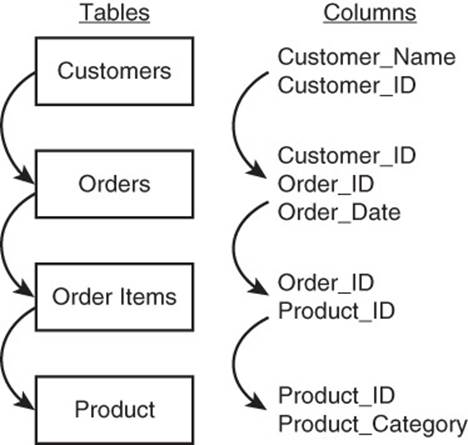
Figure 8.4 Analyzing customers who bought a particular type of product requires three joins between four tables.
To get a sense of how much work is involved in joining tables, let’s consider pseudocode for printing the name of customers who have purchased electronic accessories in the last 12 months:
for cust in get_customers():
for order in get_customer_orders(cust.customer_id):
if today() - 365 <= order.order_date:
for order_item in get_order_items
(order.order_id):
if 'electronic accessories' =
get_product_category(order_item.product_id):
customer_set = add_item
(customer_set,cust.name);
for customer_name in customer_set:
print customer_name;
In this example, the functions get_customers, get_customer_orders, and get_order_items return a list of rows. In the case of get_customers(), all customers are returned.
Each time get_customer_orders is called, it is given a customer_id. Only orders with that customer ID are returned. Each time get_order_items is called, it is given an order_id. Only order items with that order_id are returned.
The dot notation indicates a field in the row returned. For example, order.order_date returns the order_date on a particular order. Similarly, cust.name returns the name of the customer currently referenced by the cust variable.
Executing Joins Example
Now to really see how much work is involved, let’s walk through an example. Let’s assume there are 10,000 customers in the database. The first for loop will execute 10,000 times. Each time it executes, it will look up all orders for the customer. If each of the 10,000 customers has, on average, 10 orders, then the for order loop will execute 100,000 times. Each time it executes, it will check the order date.
Let’s say there are 20,000 orders that have been placed in the last year. The for order_item loop will execute 20,000 times. It will perform a check and add a customer name to a set of customer names if at least one of the order items was an electronic accessory.
Looping through rows of tables and looking for matches is one—rather inefficient—way of performing joins. The performance of this join could be improved. For example, indexes could be used to more quickly find all orders placed within the last year. Similarly, indexes could be used to find the products that are in the electronic accessory category.
Databases implement query optimizers to come up with the best way of fetching and joining data. In addition to using indexes to narrow down the number of rows they have to work with, they may use other techniques to match rows. They could, for example, calculate hash values of foreign keys to quickly determine which rows have matching values.
The query optimizer may also sort rows first and then merge rows from multiple tables more efficiently than if the rows were not sorted. These techniques can work well in some cases and not in others. Database researchers and vendors have made advances in query optimization techniques, but executing joins on large data sets can still be time consuming and resource intensive.
What Would a Document Database Modeler Do?
Document data modelers have a different approach to data modeling than most relational database modelers. Document database modelers and application developers are probably using a document database for its scalability, its flexibility, or both. For those using document databases, avoiding data anomalies is still important, but they are willing to assume more responsibility to prevent them in return for scalability and flexibility.
For example, if there are redundant copies of customer addresses in the database, an application developer could implement a customer address update function that updates all copies of an address. She would always use that function to update an address to avoid introducing a data anomaly. As you can see, developers will write more code to avoid anomalies in a document database, but will have less need for database tuning and query optimization in the future.
So how do document data modelers and application developers get better performance? They minimize the need for joins. This process is known as denormalization. The basic idea is that data models should store data that is used together in a single data structure, such as a table in a relational database or a document in a document database.
The Joy of Denormalization
To see the benefits of denormalization, let’s start with a simple example: order items and products. Recall that the Order_Items entity had the following attributes:
• order_item_ID
• order_id
• quantity
• cost_per_unit
• product_id
The Products entity has the following attributes:
• product_ID
• product_description
• product_name
• product_category
• list_price
An example of an order items document is
{
order_item_ID : 834838,
order_ID: 8827,
quantity: 3,
cost_per_unit: 8.50,
product_ID: 3648
}
An example of a product document is
{
product_ID: 3648,
product_description: "1 package laser printer paper.
100% recycled.",
product_name : "Eco-friendly Printer Paper",
product_category : "office supplies",
list_price : 9.00
}
If you implemented two collections and maintained these separate documents, then you would have to query the order items collection for the order item you were interested in and then query the products document for information about the product with product_ID 3648. You would perform two lookups to get the information you need about one order item.
By denormalizing the design, you could create a collection of documents that would require only one lookup operation. A denormalized version of the order item collection would have, for example:
{
order_item_ID : 834838,
order_ID: 8827,
quantity: 3,
cost_per_unit: 8.50,
product :
{
product_description: "1 package laser printer
paper. 100% recycled.",
product_name : "Eco-friendly Printer Paper",
product_category : "office supplies",
list_price : 9.00
}
}
![]() Note
Note
Notice that you no longer need to maintain product_ID fields. Those were used as database references (or foreign keys in relational database parlance) in the Order_Items document.
Avoid Overusing Denormalization
Denormalization, like all good things, can be used in excess. The goal is to keep data that is frequently used together in the document. This allows the document database to minimize the number of times it must read from persistent storage, a relatively slow process even when using solid state devices (SSDs). At the same time, you do not want to allow extraneous information to creep into your denormalized collection (see Figure 8.5).
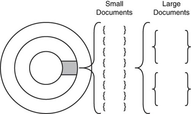
Figure 8.5 Large documents can lead to fewer documents retrieved when a block of data is read from persistent storage. This can increase the total number of data block reads to retrieve a collection or subset of collections.
To answer the question “how much denormalization is too much?” you should consider the queries your application will issue to the document database.
Let’s assume you will use two types of queries: one to generate invoices and packing slips for customers and one to generate management reports. Also, assume that 95% of the queries will be in the invoice and packing slip category and 5% of the queries will be for management reports.
Invoices and packing slips should include, among other fields, the following:
• order_ID
• quantity
• cost_per_unit
• product_name
Management reports tend to aggregate information across groups or categories. For these reports, queries would include product category information along with aggregate measures, such as total number sold. A management report showing the top 25 selling products would likely include a product description.
Based on these query requirements, you might decide it is better to not store product description, list price, and product category in the Order_Items collection. The next version of the Order_Items document would then look like this:
{
order_item_ID : 834838,
order_ID: 8827,
quantity: 3,
cost_per_unit: 8.50,
product_name : "Eco-friendly Printer Paper"
}
and we would maintain a Products collection with all the relevant product details; for example:
{
product_description: "1 package laser printer paper.
100% recycled.",
product_name : "Eco-friendly Printer Paper",
product_category : 'office supplies',
list_price : 9.00
}
Product_name is stored redundantly in both the Order_Items collection and in the Products collection. This model uses slightly more storage but allows application developers to retrieve information for the bulk of their queries in a single lookup operation.
Just Say No to Joins, Sometimes
Never say never when designing NoSQL models. There are best practices, guidelines, and design patterns that will help you build scalable and maintainable applications. None of them should be followed dogmatically, especially in the presence of evidence that breaking those best practices, guidelines, or design patterns will give your application better performance, more functionality, or greater maintainability.
If your application requirements are such that storing related information in two or more collections is an optimal design choice, then make that choice. You can implement joins in your application code. A worst-case scenario is joining two large collections with two for loops, such as
for doc1 in collection1:
for doc2 in collection2:
<do something with both documents>
If there are N documents in collection1 and M documents in collection2, this statement would execute N × M times. The execution time for such loops can grow quickly. If the first collection has 100,000 documents and the second has 500,000, then the statement would execute 50,000,000,000 (5 × 10⁵) times. If you are dealing with collections this large, you will want to use indexes, filtering, and, in some cases, sorting to optimize your join by reducing the number of overall operations performed (see Figure 8.6).
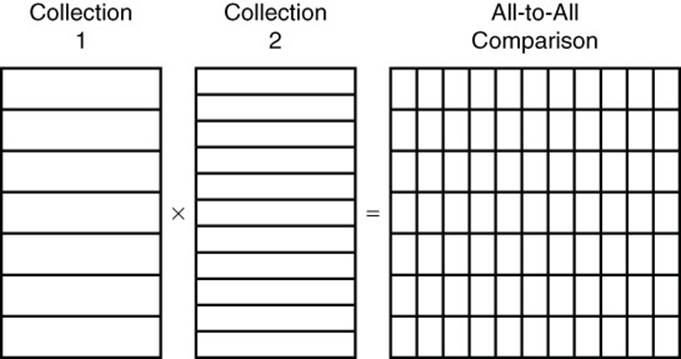
Figure 8.6 Simple join operations that compare all documents in one collection to all documents in another collection can lead to poor performance on large collections. Joins such as this can be improved by using indexes, filtering, and, in some cases, sorting.
Normalization is a useful technique for reducing the chances of introducing data anomalies. Denormalization is also useful, but for (obviously) different reasons. Specifically, denormalization is employed to improve query performance. When using document databases, data modelers and developers often employ denormalization as readily as relational data modelers employ normalization.
![]() Tip
Tip
Remember to use your queries as a guide to help strike the right balance of normalization and denormalization. Too much of either can adversely affect performance. Too much normalization leads to queries requiring joins. Too much denormalization leads to large documents that will likely lead to unnecessary data reads from persistent storage and other adverse effects.
There is another less-obvious consideration to keep in mind when designing documents and collections: the potential for documents to change size. Documents that are likely to change size are known as mutable documents.
Planning for Mutable Documents
Things change. Things have been changing since the Big Bang. Things will most likely continue to change. It helps to keep these facts in mind when designing databases.
Some documents will change frequently, and others will change infrequently. A document that keeps a counter of the number of times a web page is viewed could change hundreds of times per minute. A table that stores server event log data may only change when there is an error in the load process that copies event data from a server to the document database. When designing a document database, consider not just how frequently a document will change, but also how the size of the document may change.
Incrementing a counter or correcting an error in a field will not significantly change the size of a document. However, consider the following scenarios:
• Trucks in a company fleet transmit location, fuel consumption, and other operating metrics every three minutes to a fleet management database.
• The price of every stock traded on every exchange in the world is checked every minute. If there is a change since the last check, the new price information is written to the database.
• A stream of social networking posts is streamed to an application, which summarizes the number of posts; overall sentiment of the post; and the names of any companies, celebrities, public officials, or organizations. The database is continuously updated with this information.
Over time, the number of data sets written to the database increases. How should an application designer structure the documents to handle such input streams? One option is to create a new document for each new set of data. In the case of the trucks transmitting operational data, this would include a truck ID, time, location data, and so on:
{
truck_id: 'T87V12',
time: '08:10:00',
date : '27-May-2015',
driver_name: 'Jane Washington',
fuel_consumption_rate: '14.8 mpg',
...
}
Each truck would transmit 20 data sets per hour, or assuming a 10-hour operations day, 200 data sets per day. The truck_id, date, and driver_name would be the same for all 200 documents. This looks like an obvious candidate for embedding a document with the operational data in a document about the truck used on a particular day. This could be done with an array holding the operational data documents:
{
truck_id: 'T87V12',
date : '27-May-2015',
driver_name: 'Jane Washington',
operational_data:
[
{time : '00:01',
fuel_consumption_rate: '14.8 mpg',
...},
{time : '00:04',
fuel_consumption_rate: '12.2 mpg',
...},
{time : '00:07',
fuel_consumption_rate: '15.1 mpg',
...},
...]
}
The document would start with a single operational record in the array, and at the end of the 10-hour shift, it would have 200 entries in the array.
From a logical modeling perspective, this is a perfectly fine way to structure the document, assuming this approach fits your query requirements. From a physical model perspective, however, there is a potential performance problem.
When a document is created, the database management system allocates a certain amount of space for the document. This is usually enough to fit the document as it exists plus some room for growth. If the document grows larger than the size allocated for it, the document may be moved to another location. This will require the database management system to read the existing document and copy it to another location, and free the previously used storage space (see Figure 8.7).
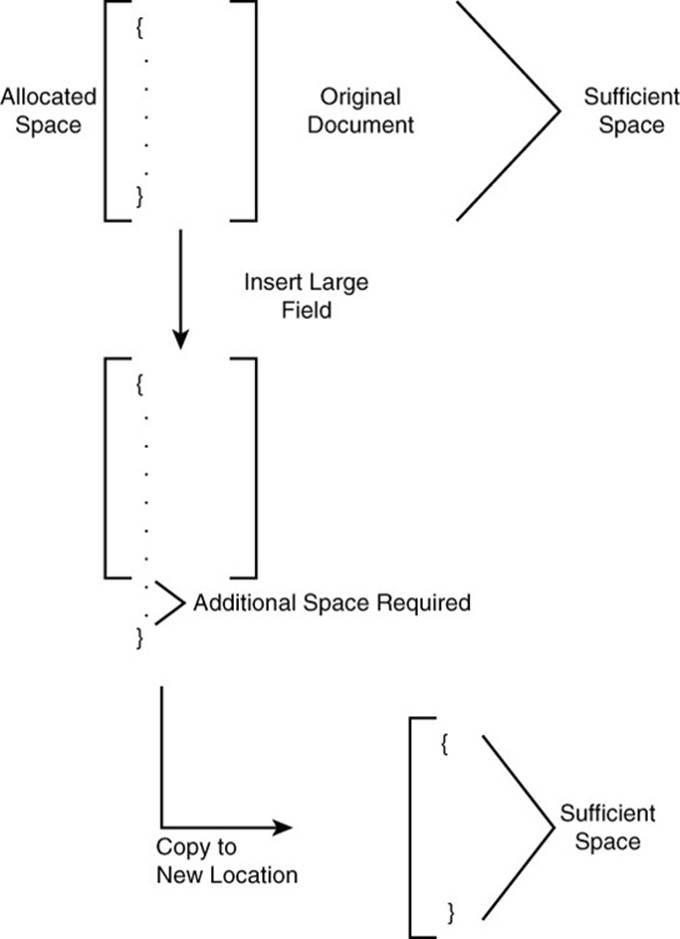
Figure 8.7 When documents grow larger than the amount of space allocated for them, they may be moved to another location. This puts additional load on the storage systems and can adversely affect performance.
Avoid Moving Oversized Documents
One way to avoid this problem of moving oversized documents is to allocate sufficient space for the document at the time the document is created. In the case of the truck operations document, you could create the document with an array of 200 embedded documents with the time and other fields specified with default values. When the actual data is transmitted to the database, the corresponding array entry is updated with the actual values (see Figure 8.8).
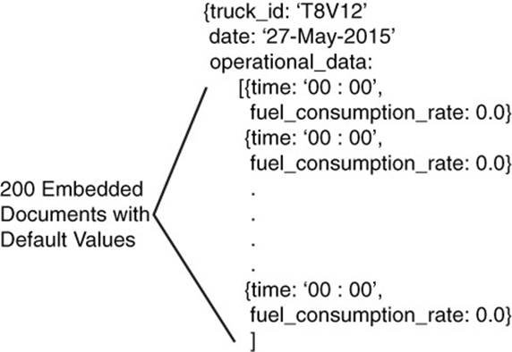
Figure 8.8 Creating documents with sufficient space for anticipated growth reduces the need to relocate documents.
Consider the life cycle of a document and when possible plan for anticipated growth. Creating a document with sufficient space for the full life of the document can help to avoid I/O overhead.
The Goldilocks Zone of Indexes
Astronomers have coined the term Goldilocks Zone to describe the zone around a star that could sustain a habitable planet. In essence, the zone that is not too close to the sun (too hot) or too far away (too cold) is just right. When you design a document database, you also want to try to identify the right number of indexes. You do not want too few, which could lead to poor read performance, and you do not want too many, which could lead to poor write performance.
Read-Heavy Applications
Some applications have a high percentage of read operations relative to the number of write operations. Business intelligence and other analytic applications can fall into this category. Read-heavy applications should have indexes on virtually all fields used to help filter results. For example, if it was common for users to query documents from a particular sales region or with order items in a certain product category, then the sales region and product category fields should be indexed.
It is sometimes difficult to know which fields will be used to filter results. This can occur in business intelligence applications. An analyst may explore data sets and choose a variety of different fields as filters. Each time he runs a new query, he may learn something new that leads him to issue another query with a different set of filter fields. This iterative process can continue as long as the analyst gains insight from queries.
Read-heavy applications can have a large number of indexes, especially when the query patterns are unknown. It is not unusual to index most fields that could be used to filter results in an analytic application (see Figure 8.9).
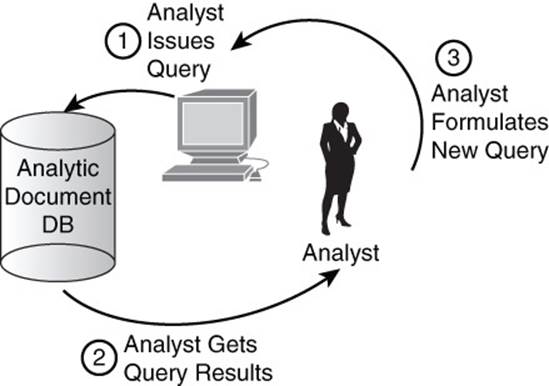
Figure 8.9 Querying analytic databases is an iterative process. Virtually any field could potentially be used to filter results. In such cases, indexes may be created on most fields.
Write-Heavy Applications
Write-heavy applications are those with relatively high percentages of write operations relative to read operations. The document database that receives the truck sensor data described previously would likely be a write-heavy database. Because indexes are data structures that must be created and updated, their use will consume CPU, persistent storage, and memory resources and increase the time needed to insert or update a document in the database.
Data modelers tend to try to minimize the number of indexes in write-heavy applications. Essential indexes, such as those created for fields storing the identifiers of related documents, should be in place. As with other design choices, deciding on the number of indexes in a write-heavy application is a matter of balancing competing interests.
Fewer indexes typically correlate with faster updates but potentially slower reads. If users performing read operations can tolerate some delay in receiving results, then minimizing indexes should be considered. If, however, it is important for users to have low-latency queries against a write-heavy database, consider implementing a second database that aggregates the data according to the time-intensive read queries. This is the basic model used in business intelligence.
Transaction processing systems are designed for fast writes and targeted reads. Data is copied from that database using an extraction, transformation, and load (ETL) process and placed in a data mart or data warehouse. The latter two types of databases are usually heavily indexed to improve query response time (see Figure 8.10).
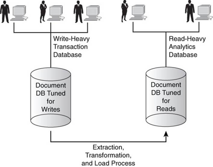
Figure 8.10 When both write-heavy and read-heavy applications must be supported, a two-database solution may be the best option.
![]() Tip
Tip
Identifying the right set of indexes for your application can take some experimentation. Start with the queries you expect to support and implement indexes to reduce the time needed to execute the most important and the most frequently executed. If you find the need for both read-heavy and write-heavy applications, consider a two-database solution with one database tuned for each type.
Modeling Common Relations
As you gather requirements and design a document database, you will likely find the need for one or more of three common relations:
• One-to-many relations
• Many-to-many relations
• Hierarchies
The first two involve relations between two collections, whereas the third can entail an arbitrary number of related documents within a collection. You learned about one-to-one and one-to-many relations previously in the discussion of normalization. At that point, the focus was on the need for joins when normalizing data models. Here, the focus is on how to efficiently implement such relationships in document databases. The following sections discuss design patterns for modeling these three kinds of relations.
One-to-Many Relations in Document Databases
One-to-many relations are the simplest of the three relations. This relation occurs when an instance of an entity has one or more related instances of another entity. The following are some examples:
• One order can have many order items.
• One apartment building can have many apartments.
• One organization can have many departments.
• One product can have many parts.
This is an example in which the typical model of document database differs from that of a relational database. In the case of a one-to-many relation, both entities are modeled using a document embedded within another document. For example:
{
customer_id: 76123,
name: 'Acme Data Modeling Services',
person_or_business: 'business',
address : [
{ street: '276 North Amber St',
city: 'Vancouver',
state: 'WA',
zip: 99076} ,
{ street: '89 Morton St',
city: 'Salem',
state: 'NH',
zip: 01097}
]
}
The basic pattern is that the one entity in a one-to-many relation is the primary document, and the many entities are represented as an array of embedded documents. The primary document has fields about the one entity, and the embedded documents have fields about the many entities.
Many-to-Many Relations in Document Databases
A many-to-many relation occurs when instances of two entities can both be related to multiple instances of another entity. The following are some examples:
• Doctors can have many patients and patients can have many doctors.
• Operating system user groups can have many users and users can be in many operating system user groups.
• Students can be enrolled in many courses and courses can have many students enrolled.
• People can join many clubs and clubs can have many members.
Many-to-many relations are modeled using two collections—one for each type of entity. Each collection maintains a list of identifiers that reference related entities. For example, a document with course data would include an array of student IDs, and a student document would include a list of course IDs, as in the following:
Courses:
{
{ courseID: 'C1667',
title: 'Introduction to Anthropology',
instructor: 'Dr. Margret Austin',
credits: 3,
enrolledStudents: ['S1837', 'S3737', 'S9825' ...
'S1847'] },
{ courseID: 'C2873',
title: 'Algorithms and Data Structures',
instructor: 'Dr. Susan Johnson',
credits: 3,
enrolledStudents: ['S1837','S3737', 'S4321', 'S9825'
... 'S1847'] },
{ courseID: C3876,
title: 'Macroeconomics',
instructor: 'Dr. James Schulen',
credits: 3,
enrolledStudents: ['S1837', 'S4321', 'S1470', 'S9825'
... 'S1847'] },
...
Students:
{
{studentID:'S1837',
name: 'Brian Nelson',
gradYear: 2018,
courses: ['C1667', C2873,'C3876']},
{studentID: 'S3737',
name: 'Yolanda Deltor',
gradYear: 2017,
courses: [ 'C1667','C2873']},
...
}
The pattern minimizes duplicate data by referencing related documents with identifiers instead of embedded documents.
Care must be taken when updating many-to-many relationships so that both entities are correctly updated. Also remember that document databases will not catch referential integrity errors as a relational database will. Document databases will allow you to insert a student document with a courseID that does not correspond to an existing course.
Modeling Hierarchies in Document Databases
Hierarchies describe instances of entities in some kind of parent-child or part-subpart relation. The product_category attribute introduced earlier is an example where a hierarchy could help represent relations between different product categories (see Figure 8.11).
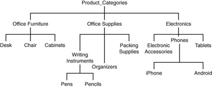
Figure 8.11 Hierarchies describe parent-child or part-subpart relations.
There are a few different ways to model hierarchical relations. Each works well with particular types of queries.
Parent or Child References
A simple technique is to keep a reference to either the parent or the children of an entity. Using the data depicted in Figure 8.11, you could model product categories with references to their parents:
{
{productCategoryID: 'PC233', name:'Pencils',
parentID:'PC72'},
{productCategoryID: 'PC72', name:'Writing Instruments',
parentID: 'PC37''},
{productCategoryID: 'PC37', name:'Office Supplies',
parentID: 'P01'},
{productCategoryID: 'P01', name:'Product Categories' }
}
Notice that the root of the hierarchy, 'Product Categories', does not have a parent and so has no parent field in its document.
This pattern is useful if you frequently have to show a specific instance and then display the more general type of that category.
A similar pattern works with child references:
{
{productCategoryID: 'P01', name:'Product Categories',
childrenIDs: ['P37','P39','P41']},
{productCategoryID: 'PC37', name:'Office Supplies',
childrenIDs: ['PC72','PC73','PC74'']},
{productCategoryID: 'PC72', name:'Writing
Instruments', childrenIDs: ['PC233','PC234']'},
{productCategoryID: 'PC233', name:'Pencils'}
}
The bottom nodes of the hierarchy, such as 'Pencils', do not have children and therefore do not have a childrenIDs field.
This pattern is useful if you routinely need to retrieve the children or subparts of the instance modeled in the document. For example, if you had to support a user interface that allowed users to drill down, you could use this pattern to fetch all the children or subparts of the current level of the hierarchy displayed in the interface.
Listing All Ancestors
Instead of just listing the parent in a child document, you could keep a list of all ancestors. For example, the 'Pencils' category could be structured in a document as
{productCategoryID: 'PC233', name:'Pencils',
ancestors:['PC72', 'PC37', 'P01']}
This pattern is useful when you have to know the full path from any point in the hierarchy back to the root.
An advantage of this pattern is that you can retrieve the full path to the root in a single read operation. Using a parent or child reference requires multiple reads, one for each additional level of the hierarchy.
A disadvantage of this approach is that changes to the hierarchy may require many write operations. The higher up in the hierarchy the change is, the more documents will have to be updated. For example, if a new level was introduced between 'Product Category' and 'Office Supplies', all documents below the new entry would have to be updated. If you added a new level to the bottom of the hierarchy—for example, below 'Pencils' you add 'Mechanical Pencils' and 'Non-mechanical Pencils'—then no existing documents would have to change.
![]() Note
Note
One-to-many, many-to-many, and hierarchies are common patterns in document databases. The patterns described here are useful in many situations, but you should always evaluate the utility of a pattern with reference to the kinds of queries you will execute and the expected changes that will occur over the lives of the documents. Patterns should support the way you will query and maintain documents by making those operations faster or less complicated than other options.
Summary
This chapter concludes the examination of document databases by considering several key issues you should consider when modeling for document databases.
Normalization and denormalization are both useful practices. Normalization helps to reduce the chance of data anomalies while denormalization is introduced to improve performance. Denormalization is a common practice in document database modeling. One of the advantages of denormalization is that it reduces or eliminates the need for joins. Joins can be complex and/or resource-intensive operations. It helps to avoid them when you can, but there will likely be times you will have to implement joins in your applications. Document databases, as a rule, do not support joins.
In addition to considering the logical aspects of modeling, you should consider the physical implementation of your design. Mutable documents, in particular, can adversely affect performance. Mutable documents that grow in size beyond the storage allocated for them may have to be moved in persistent storage, such as on disks. This need for additional writing of data can slow down your applications’ update operations.
Indexes are another important implementation topic. The goal is to have the right number of indexes for your application. All instances should help improve query performance. Indexes that would help with query performance may be avoided if they would adversely impact write performance in a noticeable way. You will have to balance benefits of faster query response with the cost of slower inserts and updates when indexes are in place.
Finally, it helps to use design patterns when modeling common relations such as one-to-many, many-to-many, and hierarchies. Sometimes embedded documents are called for, whereas in other cases, references to other document identifiers are a better option when modeling these relations.
Part IV, “Column Family Databases,” introduces wide column databases. These are another important type of NoSQL database and are especially important for managing large data sets with potentially billions of rows and millions of columns.
Case Study: Customer Manifests
Chapter 1, “Different Databases for Different Requirements,” introduced TransGlobal Transport and Shipping (TGTS), a fictitious transportation company that coordinates the movement of goods around the globe for businesses of all sizes. As business has grown, TGTS is transporting and tracking more complicated and varied shipments. Analysts have gathered requirements and some basic estimates about the number of containers that will be shipped. They found a mix of common fields for all containers and specialized fields for different types of containers.
All containers will require a core set of fields such as customer name, origination facility, destination facility, summary of contents, number of items in container, a hazardous material indicator, an expiration date for perishable items such as fruit, a destination facility, and a delivery point of contact and contact information.
In addition, some containers will require specialized information. Hazardous materials must be accompanied by a material safety data sheet (MSDS), which includes information for emergency responders who may have to handle the hazardous materials. Perishable foods must also have details about food inspections, such as the name of the person who performed the inspection, the agency responsible for the inspection, and contact information of the agency.
The analyst found that 70%–80% of the queries would return a single manifest record. These are typically searched for by a manifest identifier or by customer name, date of shipment, and originating facility. The remaining 20%–30% would be mostly summary reports by customers showing a subset of common information. Occasionally, managers will run summary reports by type of shipment (for example, hazardous materials, perishable foods), but this is rarely needed.
Executives inform the analysts that the company has plans to substantially grow the business in the next 12 to 18 months. The analysts realize that they may have many different types of cargo in the future with specialized information, just as hazardous materials and perishable foods have specialized fields. They also realize they must plan for future scaling up and the need to support new fields in the database. They concluded that a document database that supports horizontal scaling and a flexible schema is required.
The analysts start the document and collection design process by considering fields that are common to most manifests. They decided on a collection called Manifests with the following fields:
• Customer name
• Customer contact person’s name
• Customer address
• Customer phone number
• Customer fax
• Customer email
• Origination facility
• Destination facility
• Shipping date
• Expected delivery date
• Number of items in container
They also determine fields they should track for perishable foods and hazardous materials. They decide that both sets of specialized fields should be grouped into their own documents. The next question they have to decide is, should those documents be embedded with manifest documents or should they be in a separate collection?
Embed or Not Embed?
The analysts review sample reports that managers have asked for and realize that the perishable foods fields are routinely reported along with the common fields in the manifest. They decide to embed the perishable foods within the manifest document.
They review sample reports and find no reference to the MSDS for hazardous materials. They ask a number of managers and executives about this apparent oversight. They are eventually directed to a compliance officer. She explains that the MSDS is required for all hazardous materials shipments. The company must demonstrate to regulators that their database includes MSDSs and must make the information available in the event of an emergency. The compliance officer and analyst conclude they need to define an additional report for facility managers who will run the report and print MSDS information in the event of an emergency.
Because the MSDS information is infrequently used, they decide to store it in a separate collection. The Manifest collection will include a field called msdsID that will reference the corresponding MSDS document. This approach has the added benefit that the compliance officer can easily run a report listing any hazardous material shipments that do not have an msdsID. This allows her to catch any missing MSDSs and continue to comply with regulations.
Choosing Indexes
The analysts anticipate a mix of read and write operations with approximately 60%–65% reads and 35%–40% writes. They would like to maximize the speed of both reads and writes, so they carefully weigh the set of indexes to create.
Because most of the reads will be looks for single manifests, they decide to focus on that report first. The manifest identifier is a logical choice for index field because it is used to retrieve manifest doccuments.
Analysts can also look up manifests by customer name, shipment date, and origination facility. The analysts consider creating three indexes: one for each field. They realize, however, that they will rarely need to list all shipments by date or by origination facility, so they decide against separate indexes for those fields.
Instead, they create a single index on all three fields: customer name, shipment date, and origination facility. With this index, the database can determine if a manifest exists for a particular customer, shipping date, and origination facility by checking the index only; there is no need to check the actual collection of documents, thus reducing the number of read operations that have to be performed.
Separate Collections by Type?
The analysts realize that they are working with a small number of manifest types, but there may be many more in the future. For example, the company does not ship frozen goods now, but there has been discussion about providing that service. The analysts know that if you frequently filter documents by type, it can be an indicator that they should use separate collections for each type.
They soon realize they are the exception to that rule because they do not know all the types they may have. The number of types can grow quite large, and managing a large number of collections is less preferable to managing types within a single collection.
By using requirements for reports and keeping in mind some basic design principles, the analysts are able to quickly create an initial schema for tracking a complex set of shipment manifests.
Review Questions
1. What are the advantages of normalization?
2. What are the advantages of denormalization?
3. Why are joins such costly operations?
4. How do document database modelers avoid costly joins?
5. How can adding data to a document cause more work for the I/O subsystem in addition to adding the data to a document?
6. How can you, as a document database modeler, help avoid that extra work mentioned in Question 5?
7. Describe a situation where it would make sense to have many indexes on your document collections.
8. What would cause you to minimize the number of indexes on your document collection?
9. Describe how to model a many-to-many relationship.
10. Describe three ways to model hierarchies in a document database.
References
Apache Foundation. Apache CouchDB 1.6 Documentation: http://docs.couchdb.org/en/1.6.1/.
Brewer, Eric. “CAP Twelve Years Later: How the ‘Rules’ Have Changed.” Computer vol. 45, no. 2 (Feb 2012): 23–29.
Brewer, Eric A. “Towards Robust Distributed Systems.” PODC. vol. 7. 2000.
Chodorow, Kristina. 50 Tips and Tricks for MongoDB Developers. Sebastopol, CA: O’Reilly Media, Inc., 2011.
Chodorow, Kristina. MongoDB: The Definitive Guide. Sebastopol, CA: O’Reilly Media, Inc., 2013.
Copeland, Rick. MongoDB Applied Design Patterns. Sebastopol, CA: O’Reilly Media, Inc., 2013.
Couchbase. Couchbase Documentation: http://docs.couchbase.com/.
Han, Jing, et al. “Survey on NoSQL Database.” Pervasive computing and applications (ICPCA), 2011 6th International Conference on IEEE, 2011.
MongoDB. MongoDB 2.6 Manual: http://docs.mongodb.org/manual/.
O’Higgins, Niall. MongoDB and Python: Patterns and Processes for the Popular Document-Oriented Database. Sebastopol, CA: O’Reilly Media, Inc., 2011.
OrientDB. OrientDB Manual, version 2.0: http://www.orientechnologies.com/docs/last/.