NoSQL for Mere Mortals (2015)
Part IV: Column Family Databases
Chapter 11. Designing for Column Family Databases
“A good designer must rely on experience, on precise, logic thinking; and on pedantic exactness. No magic will do.”
—NIKLAUS WIRTH
COMPUTER SCIENTIST
Topics Covered In This Chapter
Guidelines for Designing Tables
Guidelines for Indexing
Tools for Working with Big Data
Case Study: Customer Data Analysis
Users drive the design of a column family database. This might seem illogical at first. After all, shouldn’t experienced designers with knowledge of the database management system take the lead on design? Actually, designers follow the lead of users. It is users who determine the questions that will be asked of the database application. They might have questions such as these:
• How many new orders were placed in the Northwest region yesterday?
• When did a particular customer last place an order?
• What orders are en route to customers in London, England?
• What products in the Ohio warehouse have fewer than the stock keeping minimum number of items?
Only when you have questions like these can you design for a column family database. Like other NoSQL databases, design starts with queries.
Queries provide information needed to effectively design column family databases. The information includes
• Entities
• Attributes of entities
• Query criteria
• Derived values
Entities represent things that can range from concrete things, such as customers and products, to abstractions such as a service level agreement or a credit score history. Entities are modeled as rows in column family databases. A single row should correspond to a single entity. Rows are uniquely identified by row keys.
Attributes of entities are modeled using columns. Queries include references to columns to specify criteria for selecting entities and to specify a set of attributes to return.
Designers use the selection criteria to determine optimal ways to organize data with tables and partitions. For example, queries that require range scans, such as selecting all orders placed between two dates, are best served by tables that order the data in the same order it will be scanned.
Designers use the set of attributes to return to help determine how to group attributes in column families. It is most efficient to store columns together that are frequently used together.
![]() Tip
Tip
When designers see queries that include derived values, such as a count of orders placed yesterday or the average dollar value of an order, it is an indication that additional attributes may be needed to store derived data.
Information about entities, attributes, query criteria, and derived values is a starting point for column family design. Designers start with this information and then use the features of column family databases to select the most appropriate implementation.
![]() Note
Note
When you first learn about column family databases, it is useful to draw parallels between relational databases and column family databases. When you have learned enough of the basics to start to design column family database applications, it is time to forget the relational analogies.
Column family databases are implemented differently than relational databases. Thinking they are essentially the same could lead to poor design decisions. It is important to understand:
• Column family databases are implemented as sparse, multidimensional maps.
• Columns can vary between rows.
• Columns can be added dynamically.
• Joins are not used; data is denormalized instead.
These characteristics of column family databases will influence design guidelines detailed in the following sections. Guidelines are presented for the major logical components of the column family database. In the case of keyspaces, there are few guidelines other than to use a separate keyspace for each application. This is based on the fact that applications will have different query patterns and, as noted previously, column family database design is largely driven by those queries.
![]() Note
Note
HBase and Cassandra are two popular column family databases. They have many features in common. They differ in others. For example, HBase uses a time stamp to keep multiple versions of column values. Cassandra uses time stamp-like data too, but for conflict resolution, not for storing multiple values. Implementation details can also vary between versions of column family database systems. What was true of an earlier version of Cassandra might not be true of the latest version.
Guidelines for Designing Tables
One of your first design decisions is to determine the tables in your schema. The following are several guidelines to keep in mind when designing tables:
• Denormalize instead of join.
• Make use of valueless columns.
• Use both column names and column values to store data.
• Model an entity with a single row.
• Avoid hotspotting in row keys.
• Keep an appropriate number of column value versions.
• Avoid complex data structures in column values.
It should be noted that some of these recommendations, such as using an appropriate number of column value versions, are not applicable to all column family database systems.
Denormalize Instead of Join
Tables model entities, so it is reasonable to expect to have one table per entity. Column family databases often need fewer tables than their relational counterparts. This is because column family databases denormalize data to avoid the need for joins. For example, in a relational database, you typically use three tables to represent a many-to-many relationship: two tables for the related entities and one table for the many-to-many relation.
Figure 11.1 shows how to model customers who bought multiple products and products that were purchased by multiple customers.
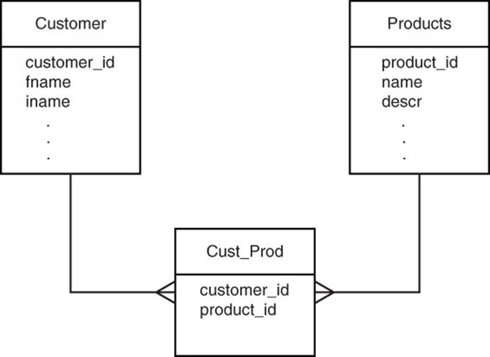
Figure 11.1 In relational databases, many-to-many relations are modeled with a table for storing primary keys of the two entities in a many-to-many relationship.
Figure 11.2 shows how to accomplish the same modeling goal with denormalized data. Each customer includes a set of column names that correspond to purchased products. Similarly, products include a list of customer IDs that indicate the set of customers that purchased those products.
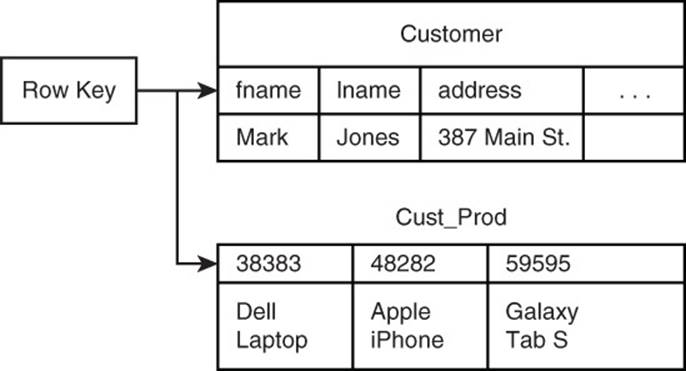
Figure 11.2 In a column family database, many-to-many relationships are captured by denormalizing data.
Make Use of Valueless Columns
You might have noticed something strange about the previous example of using column names to hold actual data about customers and products. Instead of having a column with a name like 'ProductPurchased1' with value 'PR _ B1839', the table simply stores the product ID as the column name.
![]() Tip
Tip
Using column names to store data can have advantages. For example, in Cassandra, data stored in column names is stored in sort order, but data stored in column values is not.
Of course, you could store a value associated with a column name. If a column name indicates the presence or absence of something, you could assign a T or F to indicate true or false. This, however, would take additional storage without increasing the amount of information stored in the column.
Use Both Column Names and Column Values to Store Data
A variation on the use of valueless columns uses the column value for denormalization. For example, in a database about customers and products, the features of the product, such as description, size, color, and weight, are stored in the products table. If your application users want to produce a report listing products bought by a customer, they probably want the product name in addition to its identifier. Because you are dealing with large volumes of data (otherwise you would not be using a column family database), you do not want to join or query both the customer and the product table to produce the report.
As you saw in Figure 11.2, the customer table includes a list of column names indicating the product ID of items purchased by the customer. Because the column value is not used for anything else, you can store the product name there, as shown in Figure 11.3.
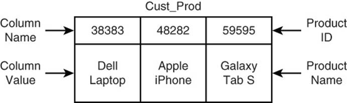
Figure 11.3 Both the column name and the column value can store data.
Keeping a copy of the product name in the customer table will increase the amount of storage used. That is one of the downsides of denormalized data. The benefit, however, is that the report of customers and the products they bought is produced by referencing only one table instead of two. In effect, you are trading the need for additional storage for improved read performance.
Model an Entity with a Single Row
A single entity, such as a particular customer or a specific product, should have all its attributes in a single row. This can lead to cases in which some rows store more column values than others, but that is not uncommon in column family databases.
Let’s consider the product table in more detail. The retailer designing the application sells several different types of products, including appliances, books, and clothing. They all share some common attributes, such as price, stock keeping unit (SKU), and inventory level. They each have unique features as well. Appliances have form factors, voltage, and energy certifications. Books have authors, publishers, and copyright dates. Clothing items have fabrics, size, and cleaning instructions. One way to model this is with several tables, as shown in Figure 11.4.
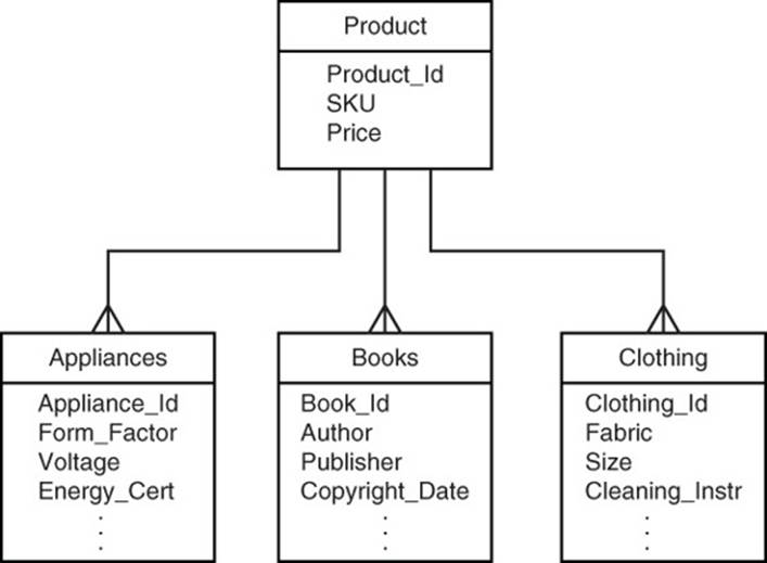
Figure 11.4 Entities can have attributes stored in multiple tables, but this is not recommended for column family databases.
Column family databases do not provide the same level of transaction control as relational databases. Typically, writes to a row are atomic. If you update several columns in a table, they will all be updated, or none of them will be.
![]() Caution
Caution
If you need to update two separate tables, such as a product table and a books table, it is conceivable the updates to the product table succeed, but the updates to the book table do not. In such a case, you would be left with inconsistent data.
Avoid Hotspotting in Row Keys
Distributed systems enable you to take advantage of large numbers of servers to solve problems. It is inefficient to direct an excessive amount of work at one or a few machines while others are underutilized.
Hotspotting occurs when many operations are performed on a small number of servers (see Figure 11.5). Consider an example of how this can occur in HBase.
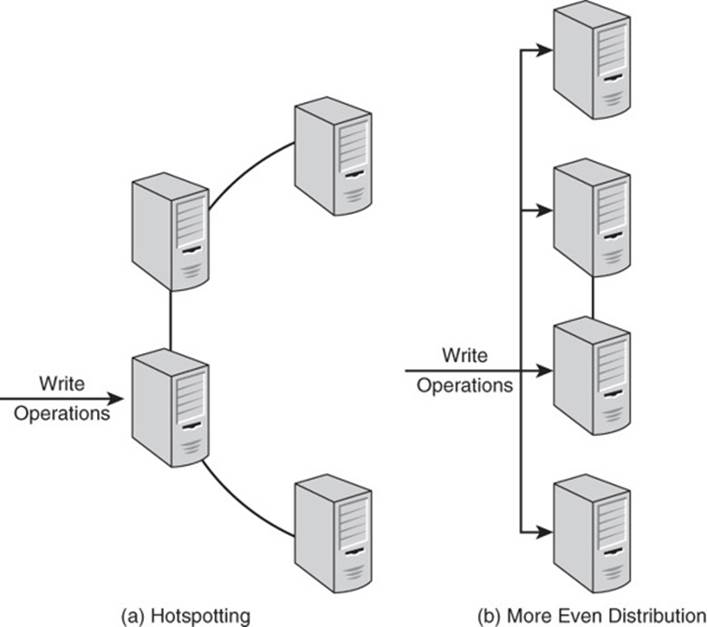
Figure 11.5 (a) Hotspotting leads to underutilization of cluster resources while (b) more even distribution of operations leads to more efficient use of resources.
HBase uses lexigraphic ordering of rows. Let’s assume you are loading data into a table and the key value for the table is a sequential number assigned by a source system. The data is stored in a file in sequential order. As HBase loads each record, it will likely write it to the same server that received the prior record and to a data block near the data block of the prior record. This helps avoid disk latency, but it means a single server is working consistently while others are underutilized.
![]() Tip
Tip
In a real-world scenario, you would probably load multiple files in parallel to utilize other servers while maintaining the benefits of reduced disk latency.
You can prevent hotspotting by hashing sequential values generated by other systems. Alternatively, you could add a random string as a prefix to the sequential value. This would eliminate the effects of the lexicographic order of the source file on the data load process.
Keep an Appropriate Number of Column Value Versions
HBase enables you to store multiple versions of a column value. Column values are time-stamped so you can determine the latest and earliest values. Like other forms of version control, this feature is useful if you need to roll back changes you have made to column values.
![]() Tip
Tip
You should keep as many versions as your application requirements dictate, but no more. Additional versions will obviously require more storage.
HBase enables you to set a minimum and maximum number of versions (see Figure 11.6). It will not remove versions if it would leave a column value with less than the minimum number of versions. When the number of versions exceeds the maximum number of versions, the oldest versions are removed during data compaction operations.
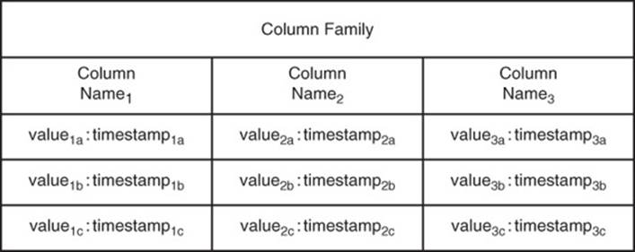
Figure 11.6 HBase provides for column value versions. The number of versions maintained is controlled by database parameters, which can be changed according to application requirements.
Avoid Complex Data Structures in Column Values
You might recall from the discussion of document databases that embedded objects are commonly used with documents. A JSON document about a customer, for example, might contain an embedded document storing address information, such as the following:
{
"customer_id":187693,
"name": "Kiera Brown",
"address" : {
"street" : "1232 Sandy Blvd.",
"city" : "Vancouver",
"state" : "Washington",
"zip" : "99121"
},
"first_order" : "01/15/2013",
"last_order" : " 06/27/2014"
}
![]() Tip
Tip
This type of data structure may be stored in a column value, but it is not recommended unless there is a specific reason to maintain this structure. If you are simply treating this object as a string and will only store and fetch it, then it is reasonable to store the string as is. If you expect to use the database to query or operate on the values within the structure, then it is better to decompose the structure.
Using separate columns for each attribute makes it easier to apply database features to the attributes. For example, creating separate columns for street, city, state, and zip means you can create secondary indexes on those values.
Also, separating attributes into individual columns allows you to use different column families if needed. Both the ability to use secondary indexes and the option of separating columns according to how they are used can lead to improved database performance.
As you can see from this discussion of guidelines for table design, there are a number of factors to consider when working with column family databases. One of the most important considerations with regard to performance is indexing.
Guidelines for Indexing
Indexes allow for rapid lookup of data in a table. For example, if you want to look up customers in a particular state, you could use a statement such as the following (in Cassandra query language, CQL):
SELECT
fname, lname
FROM
customers
WHERE
state = 'OR';
A database index functions much like the index in a book. You can look up an entry in a book index to find the pages that reference that word or term. Similarly, in column family databases, you can look up a column value, such as state abbreviation, to find rows that reference that column value. In many cases, using an index allows the database engine to retrieve data faster than it otherwise would.
It is helpful to distinguish two kinds of indexes: primary and secondary. Primary indexes are indexes on the row keys of a table. They are automatically maintained by the column family database system. Secondary indexes are indexes created on one or more column values. Either the database system or your application can create and manage secondary indexes. Not all column family databases provide automatically managed secondary indexes, but you can create and manage tables as secondary indexes in all column family database systems.
When to Use Secondary Indexes Managed by the Column Family Database System
As a general rule, if you need secondary indexes on column values and the column family database system provides automatically managed secondary indexes, then you should use them. The alternative, maintaining tables as indexes, is described in the next section.
The primary advantage of using automatically managed secondary indexes is they require less code to maintain than the alternative. In Cassandra, for example, you could create an index in CQL using the following statement:
CREATE INDEX state ON customers(state);
Cassandra will then create and manage all data structures needed to maintain the index. It will also determine the optimal use of indexes. For example, if you have an index on state and last name column values and you queried the following, Cassandra would choose which index to use first:
SELECT
fname, lname
FROM
customers
WHERE
state = 'OR'
AND
lname = 'Smith'
Typically, the database system will use the most selective index first. For example, if there are 10,000 customers in Oregon and 1,500 customers with the last name Smith, then it would use the lname secondary index first. It might then use the state index to determine, which, if any, of the 1,500 customers with the last name Smith are in Oregon.
The automatic use of secondary indexes has another major advantage because you do not have to change your code to use the indexes. Imagine you built an application according to the query requirements of your users and over time those requirements change. Now, your application has to generate a report based on state and last name instead of just state.
You could create a secondary index on the last name column and the database system would automatically use it when appropriate. As you will see in the next section, the tables as indexes method requires changes to your code.
There are times when you should not use automatically managed indexes. Avoid, or at least carefully test, the use of indexes in the following cases:
• There is a small number of distinct values in a column.
• There are many unique values in a column.
• The column values are sparse.
When the number of distinct values in a column (known as the cardinality of the column) is small, indexes will not help performance much—it might even hurt (see Figure 11.7). For example, if you have a column with values Yes and No, an index will probably not help much, especially if there are roughly equal numbers of each value.
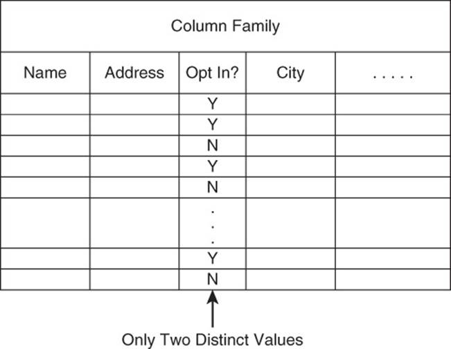
Figure 11.7 Columns with few distinct values are not good candidates for secondary indexes.
At the other end of the cardinality spectrum are columns with many distinct values, such as street addresses and email addresses (see Figure 11.8). Again, automatically managed indexes may not help much here because the index will have to maintain so much data it could take more time to search the index and retrieve the data than to scan the tables for the particular value.
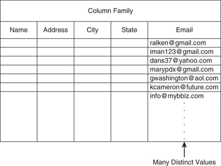
Figure 11.8 Rows with too many distinct values are also not good candidates for indexes.
In cases where many of the rows do not use a column, a secondary index may not help. For example, if most of your customers are in the United States, then their addresses will include a value in the state column. For those customers who live in Canada, they will have values in the province column instead of in the state column. Because most of your customers are in the United States, the province column will have sparse data. An index will not likely help with that column (see Figure 11.9).
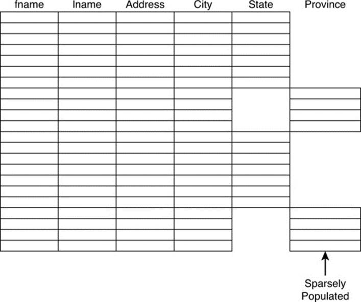
Figure 11.9 Sparsely populated columns should not be indexed.
![]() Note
Note
If you are not sure whether indexes will help, test their use if possible. Be sure to use realistically sized test data. If you create test data yourself, try to ensure it has the same range of values and distribution of values that you would see in real data. If your test data varies significantly in size or distribution, your results might not be informative for your actual use case.
A second approach to indexing is to build and manage indexes yourself using tables as indexes.
When to Create and Manage Secondary Indexes Using Tables
If your column family database system does not support automatically managed secondary indexes or the column you would like to index has many distinct values, you might benefit from creating and managing your own indexes.
Indexes created and managed by your application use the same table, column family, and column data structures used to store your data. Instead of using a statement such as CREATE INDEX to make data structures managed by the database system, you explicitly create tables to store data you would like to access via the index.
Let’s return to the customer and product database. Your end users would like to generate reports that list all customers who bought a particular product. They would also like a report on particular products and which customers bought them.
In the first situation, you would want to quickly find information about a product, such as its name and description. The existing product table meets this requirement. Next, you would want to quickly find all customers who bought that product. A time-efficient way to do this is to keep a table that uses the product identifier as the row key and uses customer identifiers as column names. The column values can be used to store additional information about the customers, such as their names. In the example shown in Figure 11.10, the necessary data is stored in the Cust _ by _ Prod table.
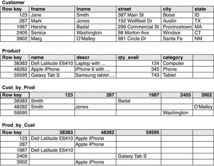
Figure 11.10 Example of tables as indexes method.
A similar approach works for the second report as well. To list all products purchased by a customer, you start with the customer table to find the customer identifier and any information about the customer needed for the report, for example, address, credit score, last purchase date, and so forth. Information about the products purchased is found in the Prod _ by _ Cust table shown in Figure 11.10.
![]() Tip
Tip
Using tables as secondary indexes will, of course, require more storage than if no additional tables were used. The same is the case when using column family database systems to manage indexes. In both cases, you are trading additional storage space for better performance.
When using tables as indexes, you will be responsible for maintaining the indexes. You have two broad options with regard to the timing of updates. You could update the index whenever there is a change to the base tables, for example, when a customer makes a purchase. Alternatively, you could run a batch job at regular intervals to update the index tables.
Updating index tables at the same time you update the base tables keeps the indexes up to date at all times. This is a significant advantage if the reports that use the index table could be run at any time. A drawback of this approach is that your application will have to perform two write operations, one to the base table and one to the index table. This could lead to longer latencies during write operations.
Updating index tables with batch jobs has the advantage of not adding additional work to write operations. The obvious disadvantage is that there is a period of time when the data in the base tables and the indexes is out of synchronization. This might be acceptable in some cases. For example, if the reports that use the index tables only run at night as part of a larger batch job, then the index tables could be updated just prior to running the report. Your reporting requirements should guide your choice of update strategy (see Figure 11.11).
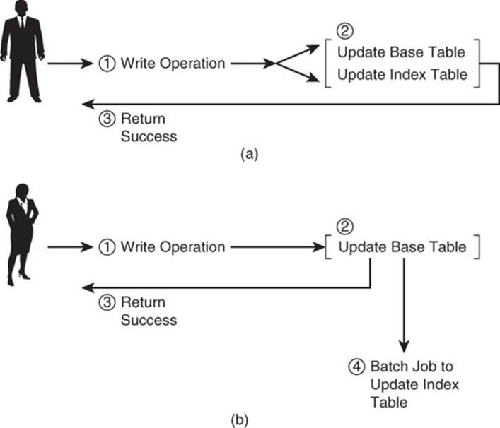
Figure 11.11 (a) Updating an index table during write operations keeps data synchronized but increases the time needed to complete a write operation. (b) Batch updates introduce periods of time when the data is not synchronized, but this may be acceptable in some cases.
Tools for Working with Big Data
NoSQL database options, such as key-value, document, and graph databases, are used with a wide range of applications with varying data sizes. Column family databases certainly could be used with small data sets, but other database types are probably better options.
![]() Note
Note
If you find yourself working with Apache HBase or Cassandra, two popular column family databases, you are probably dealing with Big Data.
The term Big Data does not have a precise definition. Informally, data sets that are too large to efficiently store and analyze in relational databases are considered Big Data. Internet search companies, such as Yahoo!, found early that relational databases would not meet the needs of a web search service. They went on to create the Hadoop platform, which is now an Apache project with broad community support.
A more formal and commonly used definition is due to the Gartner research group.1 Gartner defines Big Data as high velocity, high volume, and/or high variety. Velocity refers to the speed at which data is generated or changed. Volume refers to the size of the data. Variety refers to the range of data types and the scope of information included in the data.
1. Laney Douglas. “The Importance of ‘Big Data’: A Definition.” http://www.gartner.com/resId=2057415.
A database with information about weather, traffic, population, and cell phone use must contend with large volumes of rapidly generated data about different entities and in different forms. A column family database would be a good option for such a database.
Databases are designed to store and retrieve data, and they perform these operations well. There are, however, a number of supporting and related tasks that are usually required to get the most out of your database. These tasks include
• Extracting, transforming, and loading data (ETL)
• Analyzing data
• Monitoring database performance
Innovative designers and developers created NoSQL databases to address an emerging need. Similarly, a wide community of designers and developers has created tools to perform additional operations required to support Big Data services.
Extracting, Transforming, and Loading Big Data
Moving large amounts of data is challenging for several reasons, including
• Insufficient network throughput for the volume of data
• The time required to copy large volumes of data
• The potential for corrupting data during transmission
• Storing large amounts of data at the source and target
Data warehousing developers have faced these same problems for decades, and the challenges have gotten only more difficult with Big Data. There are many ETL tools available for data warehouse developers. Scaling ETL to Big Data volumes and variety requires attention to factors that are not common to smaller data warehouse implementations.
Examples of ETL tools for Big Data include
• Apache Flume
• Apache Sqoop
• Apache Pig
Each of these addresses particular needs in Big Data ETL and, like HBase, is part of the Hadoop ecosystem of tools.
Apache Flume is designed to move large amounts of log data, but it can be used for other types of data as well. It is a distributed system, so it has many of the benefits you have probably come to expect from such systems: reliability, scalability, and fault tolerance. It uses a streaming event model to capture and deliver data. When an event occurs, such as data is written to a log file, data is sent to Flume. Flume sends the data through a channel, which is an abstraction for delivering the data to one or more destinations.
Apache Sqoop works with relational databases to move data to and from Big Data sources, such as the Hadoop file system and to the HBase column family database. Sqoop also allows developers to run massively parallel computations in the form of MapReduce jobs.
![]() MapReduce is described in more detail in the “Tools for Analyzing Big Data” section, later in this chapter.
MapReduce is described in more detail in the “Tools for Analyzing Big Data” section, later in this chapter.
Apache Pig is a data flow language that provides a succinct way to transform data. The programming language, known as Pig Latin, has high-level statements for loading, filtering, aggregating, and joining data. Pig programs are translated into MapReduce jobs.
Analyzing Big Data
One of the reasons companies and other organizations collect Big Data is that such data holds potentially valuable insights. That is, someone can glean those insights from all the data. There are many ways to analyze data, look for patterns, and otherwise extract useful information. Two broad disciplines are useful here: statistics and machine learning.
Describing and Predicting with Statistics
Statistics is the branch of mathematics that studies how to describe large data sets, also known as populations in statistics parlance, and how to make inference from data. Descriptive statistics are particularly useful for understanding the characteristics of your data.
![]() Note
Note
Something as simple as an average and a standard deviation, which is a measure of the spread in your data, can give you a useful picture of your data, especially when comparing it with other, related data.
Figure 11.12 shows an example of the dollar value of average orders in the months of November and December. Notice that in November, the average was lower than in December and there was more variation in the size of orders. December orders have a higher average and less variation. Perhaps last-minute holiday shoppers had to purchase as much as possible from one retailer in order to finish their shopping.
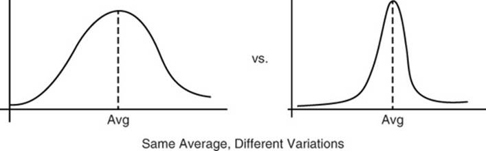
Figure 11.12 Descriptive statistics help us understand the composition of our data and how it compares with other, related data sets.
Predictive, or inferential, statistics is the study of methods for making predictions based on data (see Figure 11.13). For example, if the average December order has been increasing by 1% each year for the past 10 years, you might predict that this year’s December average will increase by 1% as well. This is a trivial example, but predictive statistics can be used for much more complex problems that include confounding factors, such as seasonal variations and differences in data set sizes.
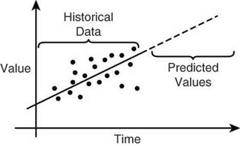
Figure 11.13 Predictive statistics help us make inferences about new situations using existing data.
![]() Note
Note
There is much more to statistics and machine learning than presented here. See the “References” section at the end of the chapter for additional resources in these areas.
Finding Patterns with Machine Learning
Machine learning is another discipline proving useful for Big Data analysis. Machine learning incorporates methods from several disciplines, including computer science, artificial intelligence, statistics, linear algebra, and others. Many services might be taken for granted, such as getting personal recommendations based on past purchases, analyzing the sentiment in social media posts, fraud detection, and machine translation, but all depend on machine-learning techniques.
One area of machine learning, called unsupervised learning, is useful for exploring large data sets. A common unsupervised learning method is clustering. Clustering algorithms are helpful when you want to find nonapparent structures or common patterns in data. For example, your company may have a cluster of customers who tend to shop late at night and early in the week. Marketing professionals can devise incentives targeted at this particular group to increase the average dollar value of their purchases.
Supervised learning techniques provide the means to learn from examples. A credit card company, for example, has large volumes of data on legitimate credit card transactions as well as data on fraudulent transactions. There are many ways to use this data to create classifiers, which are programs that can analyze transactions and classify them as either legitimate or fraudulent.
Tools for Analyzing Big Data
NoSQL database users have the option of using freely available distributed platforms for building their own tools or using available statistics and machine-learning tools. Four widely used tools are
• MapReduce
• Spark
• R
• Mahout
MapReduce and Spark are distributed platforms. R is a widely used statistics package, and Mahout is a machine-learning system designed for Big Data.
MapReduce is a programming model used for distributed, parallel processing. MapReduce programs consist of two primary components: a mapping function and a reducing function. The MapReduce engine applies the mapping function to a set of input data to generate a stream of output values. Those values are then transformed by a reducing function, which often performs aggregating operations, like counting, summing, or averaging the input data. The MapReduce model is a core part of the Apache Hadoop project and is widely used for Big Data analysis.
Spark is another distributed computational platform. Spark was designed by researchers at the University of California, Berkley, as an alternative to MapReduce. Both are designed to solve similar types of problems, but they take different approaches. MapReduce writes much data to disk, whereas Spark makes more use of memory. MapReduce employs a fairly rigid computational model (map operation followed by reduce operation), whereas Spark allows for more general computational models.
R is an open source statistics platform. The core platform contains modules for many common statistical functions. Libraries with additional capabilities are added to the R environment as needed by users. Libraries are available to support machine learning and data mining, specialized disciplines (for example, aquatic sciences), visualization, and specialized statistical methods. R did not start out as a tool for Big Data, but at least two libraries are available that support Big Data analysis.
Mahout is an Apache project developing machine-learning tools for Big Data. Mahout machine-learning packages were originally written as MapReduce programs, but newer implementations are using Spark. Mahout is especially useful for recommendations, classification, and clustering.
Tools for Monitoring Big Data
One of the primary responsibilities of system administrators is ensuring applications and servers are running as expected. When an application runs on a cluster of servers instead of a single server, the system administrator’s job is even more difficult. General cluster-monitoring tools and database-specific tools can help with distributed systems management. Examples of these tools are
• Ganglia
• Hannibal for HBase
• OpsCenter for Cassandra
Ganglia is monitoring tool designed for high-performance clusters. It is not specific to any one type of database. It uses a hierarchical model to represent nodes in a cluster and manage communication between nodes. Ganglia is a freely available open source tool.
Hannibal is an open source monitoring tool for HBase. It is especially useful for monitoring and managing regions, which are high-level data structures used in distributing data. Hannibal includes visualization tools that allow administrators to quickly assess the current and historical state of data distribution in the cluster.
OpsCenter is another open source tool, but it is designed for the Cassandra database. OpsCenter gives system administrators a single point of access to information about the state of the cluster and jobs running on the cluster.
Summary
Column family databases are designed for large volumes of data. They are flexible in regard to the type of data stored and the structure of schemas. Although you will find a good amount of overlap in terminology between relational database and column family databases, the similarity is only superficial. Column family databases optimize storage by using efficient data structures for sparse, multidimensional data sets.
To get the most out of your column family database, it is important to work with, and not against, the data structures and processes that implement the column family database. Guidelines outlined in this chapter can help when designing tables, column families, and columns.
The discussion of indexes demonstrates a common choice developers and designers face: Which is more important, time or space? When time—as in query response time—is important, use indexes. Column family databases automatically index on row keys. When you need secondary indexes on column values and your database system does not support them, you can implement your own indexes using tables. There are some disadvantages to this approach compared with database-supported secondary indexes, but the benefits often outweigh the disadvantages.
If you find yourself using a column family database, you are probably working with Big Data. It helps to use tools designed specifically for moving, processing, and managing Big Data and Big Data systems.
Case Study: Customer Data Analysis
Chapter 1, “Different Databases for Different Requirements,” introduced TransGlobal Transport and Shipping (TGTS), a fictitious transportation company that coordinates the movement of goods around the globe for businesses of all sizes. Chapter 8, “Designing for Document Databases,” discussed how the shipping company could use document databases to help manage shipping manifests.
The following case study applies concepts you learned in this chapter to show how TGTS can use column family databases to store and analyze large volumes of data about its customers and their shipping practices.
Understanding User Needs
Analysts at TGTS would like to understand how customer shipping patterns are changing. The analysts have several hypotheses about why some customers are shipping more and others are shipping less. They would like to have a large data store with a wide range of data, including
• All shipping orders for all customers since the start of the company
• All details kept in customer records
• News articles, industry newsletters, and other text on their customers’ industries and markets
• Historical data about the shipping industry, especially financial databases
The variety and volume of data put this project into the Big Data category, so the development team decides to use a column family database. Next, they turn their attention to specific query requirements.
In the first phase of the project, analysts want to apply statistical and machine-learning techniques to get a better sense of the data. Questions include: Are there clusters of similar customers or shipping orders? How does the average value of order vary by customer and by time of year the shipment is made? They also want to run reports on specific customers and shipping routes. The queries for these reports are
• For a particular customer, what orders have been placed?
• For a particular order, what items were shipped?
• For a particular route, how many ships used that route in a given time period?
• For customers in a particular industry, how many shipments were made during a particular period of time?
The database designers have a good sense of the entities that need to be modeled in the first phase of the project. The column store database will need tables for
• Customers
• Orders
• Ships
• Routes
Customers will have a single column family with data about company name, addresses, contacts, industry, and market categories. Orders will have details about items shipped, such as names, descriptions, and weights. Ships will have details about the capacity, age, maintenance history, and other features of the vessels. Routes will store descriptive information about routes as well as geographic details of the route.
In addition to the tables for the four primary entities, the designers will implement tables as indexes for the following:
• Orders by customer
• Shipped items by order
• Ships by route
The tables as indexes allow for rapid retrieval of data as needed by the queries. Because these reports are run after data is loaded in batch, it is not a problem if the base tables and tables as indexes are not synchronized for some time during the load.
In addition, because some of the queries make a reference to a period of time, the designers will implement database-managed indexes on data columns. This will allow developers and users to issue queries and filter by date without having to use specialized index tables.
Review Questions
1. What is the role of end-user queries in column family database design?
2. How can you avoid performing joins in column family databases?
3. Why should entities be modeled in a single row?
4. What is hotspotting, and why should it be avoided?
5. What are some disadvantages of using complex data structures as a column value?
6. Describe three scenarios in which you should not use secondary indexes.
7. What are the disadvantages of managing your own tables as indexes?
8. What are two types of statistics? What are they each used for?
9. What are two types of machine learning? What are they used for?
10. How is Spark different from MapReduce?
References
Apache Cassandra Glossary: http://io.typepad.com/glossary.html
Apache HBase Reference Guide: http://hbase.apache.org/book.html
Bishop, Christopher M. Pattern Recognition and Machine Learning. vol. 4. no. 4. New York: Springer, 2006.
Chang, Fay, et al. “BigTable: A Distributed Storage System for Structured Data.” OSDI’06: Seventh Symposium on Operating System Design and Implementation, Seattle, WA, November, 2006. http://research.google.com/archive/bigtable.html
FoundationDB. “ACID Claims.” https://foundationdb.com/acid-claims
Hewitt, Eben. Cassandra: The Definitive Guide. Sebastopol, CA: O’Reilly Media, Inc., 2010.
Pedregosa, Fabian, et al. “Scikit-learn: Machine Learning in Python.” The Journal of Machine Learning Research 12 (2011): 2825–2830.
Ratner, Bruce. Statistical and Machine-Learning Data Mining: Techniques for Better Predictive Modeling and Analysis of Big Data. Boca Raton: CRC Press, 2011.
Rice University, University of Houston Clear Lake, and Tufts University. “Online Statistics Education: An Interactive Multimedia Course of Study”: http://onlinestatbook.com/
Wikibooks. “Statistics.” http://en.wikibooks.org/wiki/Statistics
All materials on the site are licensed Creative Commons Attribution-Sharealike 3.0 Unported CC BY-SA 3.0 & GNU Free Documentation License (GFDL)
If you are the copyright holder of any material contained on our site and intend to remove it, please contact our site administrator for approval.
© 2016-2026 All site design rights belong to S.Y.A.