Expert Oracle SQL: Optimization, Deployment, and Statistics (2014)
PART 2. Advanced Concepts
CHAPTER 9. Object Statistics
Although the CBO makes its decisions about how to optimize a statement using data from various sources, the majority of the important information the CBO needs comes from object statistics. Most of this chapter is dedicated to an explanation of object statistics, although we will conclude this chapter with a few short points about other sources of information that the CBO uses.
In principle, and largely in practice, the use of object statistics as the basis for optimization is ideal. For example, we need some way to distinguish a tiny configuration table with ten rows from a transactional table with terabytes of data—object statistics can do that for us. Notice that if the CBO was designed to get its input from the actual size of a table, rather than a separate statistic, we would have no way to control changes to the CBO input data; every time we added a row to a table the execution plan for a statement might change.
We can categorize object statistics in two ways: by object type and by level. We have table statistics, index statistics, and column statistics, and for each table, column, or index, we may hold data at the global, partition, or subpartition level.
![]() Note If you use domain indexes you can create your own object statistics types. For details see the Data Cartridge Developer’s Guide. There are also various statistics associated with user-defined object types and object tables. For information see the Object-Relational Developer’s Guide. I will not be covering domain indexes or object-relational concepts in this book.
Note If you use domain indexes you can create your own object statistics types. For details see the Data Cartridge Developer’s Guide. There are also various statistics associated with user-defined object types and object tables. For information see the Object-Relational Developer’s Guide. I will not be covering domain indexes or object-relational concepts in this book.
This chapter will explain what each statistic is and how it is used, as well as explain why we have three different levels of statistics. But I would like to begin by making some general points about the application of object statistics and explaining how they are obtained in the first place.
The Purpose of Object Statistics
Let us assume that the CBO is considering accessing a table using a full table scan (FTS). There are three crucial metrics that the CBO needs to estimate:
· Cost. In other words, the CBO needs to know how long the FTS is likely to take. If it is quick then the FTS may be a good idea and if it takes ages then maybe not.
· Cardinality. When deciding whether to do an FTS or use an index to access a table, the number of rows returned isn’t directly relevant; the same number of rows will be returned no matter how we access the table. On the other hand, the number of rows input to theparent operation may be of crucial importance. For example, suppose that the result of the FTS is then used as the driving row source of a join with another row source. If the FTS returns only one or two rows then a nested loop may be a good idea. If the FTS returns 10,000 rows then maybe a hash join would be better. The cardinality of an FTS can be determined in two stages. First, we need to know the number of rows in the table, and second, we need to know the selectivity of the predicates. So, for example, if a table has 1,000 rows and we have a 10% selectivity (otherwise expressed as a selectivity of 0.1) then the number of rows returned by the full table scan will be 10% of 1,000, i.e., 100.
· Bytes.Like cardinality, the number of bytes returned by a table access will be the same no matter whether an FTS or an index is used. However, if the CBO wants to perform a hash join on two tables, each with 10,000 rows, then the driving row source will be selected based on the smaller of the two tables as measured in bytes.
Although I have used an FTS as my example, the same three metrics are critical to all row-source operations, and the main purpose of object statistics is to help the CBO estimate them as accurately as possible.
In a small number of cases, most notably when accessing a table through an index, estimates for multiple row-source operations need to be obtained together. We will consider this special case as part of our discussion of the clustering factor index statistic shortly.
Creating Object Statistics
The CBO reads object statistics from the data dictionary, but these statistics need to be put into the data dictionary in the first place. There are four different ways to create or update object statistics using the DBMS_STATS package: gathering, importing, transferring, and setting statistics. Furthermore:
· By default, object statistics are generated for an index when it is created or rebuilt.
· By default, in database release 12cR1 onwards, object statistics for a table and its associated columns are generated when a table is created with the CREATE TABLE ... AS SELECT option or when an empty table is loaded in bulk with an INSERT statement.
Let me go through these options one at a time.
Gathering Object Statistics
Gathering statistics is by far the most common way to create or update statistics, and for application objects one of four different procedures from the DBMS_STATS package needs to be used:
· DBMS_STATS.GATHER_DATABASE_STATS gathers statistics for the entire database.
· DBMS_STATS.GATHER_SCHEMA_STATS gathers statistics for objects within a specified schema.
· DBMS_STATS.GATHER_TABLE_STATS gathers statistics for a specified table, table partition, or table subpartition.
· When statistics are gathered for a partitioned table it is possible to gather them for all partitions and subpartitions, if applicable, as part of the same call.
· Whether statistics are gathered for a table, partition, or subpartition the default behavior is to gather statistics for all associated indexes as part of the same call.
· In addition to table statistics, this procedure gathers statistics for some or all columns in the table at the same time; there is no option to gather column statistics separately.
· DBMS_STATS.GATHER_INDEX_STATS gathers statistics for a specified index, index partition, or index subpartition. As with DBMS_STATS.GATHER_TABLE_STATS it is possible to gather statistics at the global, partition, and subpartition level as part of the same call.
![]() Note Objects in the data dictionary also need object statistics. These are obtained using the DBMS_STATS.GATHER_DICTIONARY_STATS and DBMS_STATS.GATHER_FIXED_OBJECT_STATS procedures.
Note Objects in the data dictionary also need object statistics. These are obtained using the DBMS_STATS.GATHER_DICTIONARY_STATS and DBMS_STATS.GATHER_FIXED_OBJECT_STATS procedures.
All the statistics-gathering procedures in the DBMS_STATS work in a similar way: the object being analyzed is read using recursive SQL statements. Not all blocks in the object need be read. By default, data is randomly sampled until DBMS_STATS thinks that additional sampling will not materially affect the calculated statistics. The logic to determine when to stop is remarkably effective in release 11gR1 onward in the vast majority of cases.
![]() Note In some cases, such as when you have a column that has the same value for 2,000,000 rows and a second value for 2 rows, the random sampling is likely to prematurely determine that all the rows in the table have the same value for the column. In such cases, you should simply set the column statistics to reflect reality!
Note In some cases, such as when you have a column that has the same value for 2,000,000 rows and a second value for 2 rows, the random sampling is likely to prematurely determine that all the rows in the table have the same value for the column. In such cases, you should simply set the column statistics to reflect reality!
There are a lot of optional parameters to the DBMS_STATS statistics-gathering procedures. For example, you can indicate that statistics should only be gathered on an object if they are missing or deemed to be stale. You can also specify that statistics gathering is done in parallel. For more details see the PL/SQL Packages and Types Reference manual.
You should be aware that when Oracle database is first installed a job to gather statistics for the database as a whole is automatically created. I suspect this job is there to cater to the not insubstantial number of customers that never think about object statistics. For most large-scale systems, customization of this process is necessary and you should review this job carefully. The job is scheduled in a variety of different ways depending on release, so for more details see the SQL Tuning Guide (or the Performance Tuning Guide for release 11g or earlier).
In the vast majority of cases, the initial set of statistics for an object should be gathered. It is the only practical way. On the other hand, as I explained in Chapter 6, statistics gathering on production systems should be kept to a minimum. I am now going to explain one way in which statistics gathering on a production system can be eliminated altogether.
Exporting and Importing Statistics
If you are a fan of cooking shows you will be familiar with expressions like “here is one that I created earlier.” Cooking takes time and things sometimes go wrong. So on TV cooking shows it is normal, in the interest of time, to show the initial stages of preparing a meal and then shortcut to the end using a pre-prepared dish.
In some ways, gathering statistics is like cooking: it takes some time and a small slip-up can ruin things. The good news is that DBAs, like TV chefs, can often save time and avoid risk by importing pre-made statistics into a database. The use of pre-made statistics is one of a few key concepts in the TSTATS deployment approach that I introduced in Chapter 6, but there are many other scenarios where the use of pre-made object statistics is useful. One such example is a lengthy data conversion, migration, or upgrade procedure. Such procedures are often performed in tight maintenance windows and rehearsed several times using data that, if not identical to production, are very similar. Object statistics derived from this test data may very well be suitable for use on the production system. Listing 9-1 demonstrates the technique.
Listing 9-1. Copying statistics from one system to another using DBMS_STATS export and import procedures
CREATE TABLE statement
(
transaction_date_time TIMESTAMP WITH TIME ZONE
,transaction_date DATE
,posting_date DATE
,posting_delay AS (posting_date - transaction_date)
,description VARCHAR2 (30)
,transaction_amount NUMBER
,amount_category AS (CASE WHEN transaction_amount < 10 THEN 'LOW'
WHEN transaction_amount < 100 THEN 'MEDIUM' ELSE 'HIGH'
END)
,product_category NUMBER
,customer_category NUMBER
)
PCTFREE 80
PCTUSED 10;
INSERT INTO statement (transaction_date_time
,transaction_date
,posting_date
,description
,transaction_amount
,product_category
,customer_category)
SELECT TIMESTAMP '2013-01-01 12:00:00.00 -05:00'
+ NUMTODSINTERVAL (TRUNC ( (ROWNUM - 1) / 50), 'DAY')
,DATE '2013-01-01' + TRUNC ( (ROWNUM - 1) / 50)
,DATE '2013-01-01' + TRUNC ( (ROWNUM - 1) / 50) + MOD (ROWNUM, 3)
posting_date
,DECODE (MOD (ROWNUM, 4)
,0, 'Flight'
,1, 'Meal'
,2, 'Taxi'
,'Deliveries')
,DECODE (MOD (ROWNUM, 4)
,0, 200 + (30 * ROWNUM)
,1, 20 + ROWNUM
,2, 5 + MOD (ROWNUM, 30)
,8)
,TRUNC ( (ROWNUM - 1) / 50) + 1
,MOD ( (ROWNUM - 1), 50) + 1
FROM DUAL
CONNECT BY LEVEL <= 500;
CREATE INDEX statement_i_tran_dt
ON statement (transaction_date_time);
CREATE INDEX statement_i_pc
ON statement (product_category);
CREATE INDEX statement_i_cc
ON statement (customer_category);
BEGIN
DBMS_STATS.gather_table_stats (
ownname => SYS_CONTEXT ('USERENV', 'CURRENT_SCHEMA')
,tabname => 'STATEMENT'
,partname => NULL
,granularity => 'ALL'
,method_opt => 'FOR ALL COLUMNS SIZE 1'
,cascade => FALSE);
END;
/
BEGIN
DBMS_STATS.create_stat_table (
ownname => SYS_CONTEXT ('USERENV', 'CURRENT_SCHEMA')
,stattab => 'CH9_STATS');
DBMS_STATS.export_table_stats (
ownname => SYS_CONTEXT ('USERENV', 'CURRENT_SCHEMA')
,tabname => 'STATEMENT'
,statown => SYS_CONTEXT ('USERENV', 'CURRENT_SCHEMA')
,stattab => 'CH9_STATS');
END;
/
-- Move to target system
BEGIN
DBMS_STATS.delete_table_stats (
ownname => SYS_CONTEXT ('USERENV', 'CURRENT_SCHEMA')
,tabname => 'STATEMENT');
DBMS_STATS.import_table_stats (
ownname => SYS_CONTEXT ('USERENV', 'CURRENT_SCHEMA')
,tabname => 'STATEMENT'
,statown => SYS_CONTEXT ('USERENV', 'CURRENT_SCHEMA')
,stattab => 'CH9_STATS');
END;
/
· Listing 9-1 creates a table called STATEMENT that will form the basis of other demonstrations in this chapter. STATEMENT is loaded with data, some indexes are created, and then statistics are gathered. At this stage you have to imagine that this table is on the source system, i.e., the test system in the scenario I described above.
· The first stage in the process of statistics copying is to create a regular heap table to hold the exported statistics. This has to have a specific format and is created using a call to DBMS_STATS.CREATE_STAT_TABLE. I have named the heap table CH9_STATS, but I could have used any name.
· The next step is to export the statistics. I have done so using DBMS_STATS.EXPORT_TABLE_STATS that by default exports statistics for the table, its columns, and associated indexes. As you might imagine, there are variants of this procedure for the database and schema, amongst others.
· The next step in the process is not shown but involves moving the heap table to the target system, i.e., the production system in the scenario I described above. This could be done by use of a database link or with the datapump utility. However, my preferred approach is to generate either a SQL Loader script or just a bunch of INSERT statements. This allows the script to be checked into a source-code control system along with other project scripts for posterity.
· You now have to imagine that the remaining code in Listing 9-1 is running on the target system. It is good practice to delete any existing statistics on your target table or tables using DBMS_STATS.DELETE_TABLE_STATS orDBMS_STATS.DELETE_SCHEMA_STATS first. Otherwise you may end up with a hybrid set of statistics.
· A call to DBMS_STATS.IMPORT_TABLE_STATS is then performed to load object statistics from the CH9_STATS heap table into the data dictionary, where the CBO can then use them for SQL statements involving the STATEMENT table.
In case there is any doubt, the time that these export/import operations take bears no relation to the size of the objects concerned. The time taken to perform export/import operations is purely the result of the number of objects involved, and for most databases importing statistics is a task that can be completed within a couple of minutes at most.
Transferring Statistics
Oracle database 12cR1 introduced an alternative to the export/import approach for copying statistics from one database to another. The DBMS_STATS.TRANSFER_STATS procedure allows object statistics to be copied without having to create a heap table, such as CH9_STATS used byListing 9-1. Listing 9-2 shows how to transfer statistics for a specific table directly from one database to another.
Listing 9-2. Transferring statistcs between databases using a database link
BEGIN
DBMS_STATS.transfer_stats (
ownname => SYS_CONTEXT ('USERENV', 'CURRENT_SCHEMA')
,tabname => 'STATEMENT'
,dblink => 'DBLINK_NAME');
END;
/
If you want to try this you will need to replace the DBLINK_NAME parameter value with the name of a valid database link on your target database that refers to the source database. The statistics for the table STATEMENT will be transferred directly from one system to another.
Perhaps I am a little old fashioned, but it seems to me that if your statistics are important enough to warrant copying then they are worth backing up. On that premise, the approach in Listing 9-1 is superior to that in Listing 9-2. But then again, maybe you just can’t teach an old dog new tricks.
Setting Object Statistics
Although the vast majority of object statistics should be gathered, there are a few occasions where statistics need to be directly set. Here are a few of them:
· Users of the DBMS_STATS.COPY_TABLE_STATS package may need to set statistics for some columns for the partition that is the target of the copy. We will discuss DBMS_STATS.COPY_TABLE_STATS in Chapter 20.
· The TSTATS deployment model requires the minimum and maximum values of columns to be deleted for some columns. The TSTATS model for stabilizing execution plans will also be discussed in Chapter 20.
· Gathering statistics on temporary tables can be tricky because at the time that statistics are gathered the temporary table is likely to be empty, particularly when ON COMMIT DELETE ROWS is set for the table.
· In my opinion, histograms should be manually set on all columns that require them. I advocate manually setting histograms so that the number of test cases is limited. Listing 9-8 later in this chapter gives an example of how to directly set up histograms and explains the benefits in more detail.
Creating or Rebuilding Indexes and Tables
Gathering object statistics on large indexes can be a time-consuming affair because data needs to be read from the index. However, statistics for an index can be generated as the index is being built or rebuilt with virtually no additional overhead. and this is the default behavior unless statistics for the table being indexed are locked. Notice that this behavior cannot be suppressed even when an index is being created for an empty table that is yet to be loaded.
It is also possible to generate table and column statistics when a CREATE TABLE ... AS SELECT statement is run and when data is bulk loaded into an empty table using SQL Loader, or by using an INSERT ... SELECT statement. Curiously, the ability to generate statistics for a table during creation or loading did not appear until 12cR1. Here are some general tips applicable to 12cR1 and later:
· When statistics are generated by a bulk data load, no column histograms are generated and the statistics for any indexes are not updated.
· Statistics can be generated for bulk loads into non-empty tables by use of the GATHER_OPTIMIZER_STATISTICS hint.
· Statistic generation for CREATE TABLE ... AS SELECT statements and bulk loading of empty tables can be suppressed by the NO_GATHER_OPTIMIZER_STATISTICS hint.
The above rules might lead you to believe that if you load data in bulk and then create indexes then you will not need to gather any more statistics. However, function-based indexes add hidden columns to a table, and the statistics for these columns can only be obtained after the indexes are created. There are also complications involving partitioning and indexed organized tables. For precise details of how and when objects statistics are gathered during table creation and bulk inserts please refer to the SQL Tuning Guide.
Creating Object Statistics Wrap Up
I have now explained five different ways that object statistics can be loaded into the data dictionary. The primary mechanism is to gather object statistics directly using procedures such as DBMS_STATS.GATHER_TABLE_STATS. We can also load pre-made statistics usingDBMS_STATS.IMPORT_TABLE_STATS or DBMS_STATS.TRANSFER_STATS. A fourth option is to set the object statistics to specific values using procedures such as DBMS_STATS.SET_TABLE_STATS. Finally, object statistics may be generated by DDL or DML operations, such asCREATE INDEX.
Now that we have loaded our object statistics into the database it would be nice to be able to look at them. Let us deal with that now.
Examining Object Statistics
Object statistics are held both in the data dictionary and in tables created by DBMS_STATS.CREATE_STAT_TABLE. Let us see how we can find and interpret these statistics, beginning with the data dictionary.
Examining Object Statistics in the Data Dictionary
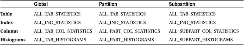
Statistics in the data dictionary can be obtained by calls to procedures in the DBMS_STATS package, such as DBMS_STATS.GET_COLUMN_STATS. However, it is generally more convenient to use views on the data dictionary. Table 9-1 lists the primary views for examining object statistics.
Table 9-1. Views for examining object statistics in the data dictionary
At this point I need to define some terms to avoid confusion.
· Object statistics are associated with a table, index, or column. In this chapter I will use the terms object table, object index, and object column when referring to entities that have object statistics. My use of these terms in this chapter is unrelated to their normal use as defined in the Object-Relational Developer’s Guide.
· Object statistics can be displayed using the views in Table 9-1, among others. I will refer to such a view as a statistic view and a column in a statistic view as statistic column.
· I will use the term export table to refer to a table created by DBMS_STATS.CREATE_STAT_TABLE. I will use the term export column to refer to a column in an export table.
![]() Tip Although the normal way to load data into an export table is with DBMS_STATS.EXPORT_TABLE_STATS it is also possible to use procedures such as DBMS_STATS.GATHER_TABLE_STATS to gather statistics directly into export tables without updating the data dictionary.
Tip Although the normal way to load data into an export table is with DBMS_STATS.EXPORT_TABLE_STATS it is also possible to use procedures such as DBMS_STATS.GATHER_TABLE_STATS to gather statistics directly into export tables without updating the data dictionary.
Consider the following when looking at Table 9-1:
· Histograms are a special type of column statistic. Unlike other types of column statistic, more than one row in the statistic view is required for each object column. Because of this, histograms are shown in a separate set of statistic views than other column statistics.
· The views listed in Table 9-1 all begin with ALL. As with many data dictionary views there are alternative variants prefixed by USER and DBA. USER views just list statistics for objects owned by the current user. Suitably privileged users have access to DBA variants that include objects owned by SYS and other objects that the current user does not have access to. The views in Table 9-1 begin with ALL and display object statistics for all objects that the current user has access to, including objects owned by other users. Objects that the current user has no access to are not displayed.
· Object statistics are included in many other common views, such as ALL_TABLES, but these views may be missing some key columns. For example, the column STATTYPE_LOCKED indicates whether statistics for a table are locked, and this column is not present inALL_TABLES; it is present in ALL_TAB_STATISTICS.
· The view ALL_TAB_COL_STATISTICS excludes object columns that have no statistics, and the three histogram statistic views do not necessarily list all object columns. The other eight tables in Listing 9-1 include rows for objects that have statistics and for objects that have no statistics.
Examining Exported Object Statistics
When you look at an export table you will see that most export columns have deliberately meaningless names. For example, in an export table created in 11gR2 there are 12 numeric columns with names from N1 to N12. There are two columns of type RAW named R1 and R2, 30-byte character columns named C1 to C5, and columns CH1, CL1, and D1. These last three columns are a 1000-byte character column, a CLOB, and a DATE respectively. Additional columns have been added in 12cR1.
All sorts of statistics can be held in export tables, not just object statistics, and these meaningless column names reflect the multi-purpose nature of an export table. Theoretically, you shouldn’t need to interpret the data in such tables. Unfortunately, in practice you may well have to. One common scenario that involves manipulating exported statistics directly involves partitioned tables. Suppose you take a backup of partition-level statistics for a table partitioned by date and want to restore these statistics a year later. Some partitions will have been dropped and others created and so the names of the partitions will likely have changed. The most practical thing to do is just to update the names of the partitions in the export table before importing.
There are some columns in an export table that have meaningful, or semi-meaningful, names:
· TYPE indicates the type of statistic. T means table, I means index, and C indicates that the row holds column statistics. When an object column has histograms there are multiple rows in the export table for the same object column. All such rows in the export table have a TYPE of C.
· FLAGS is a bitmask. For example, if the value of TYPE is C and FLAGS is odd (the low order bit is set), the statistics for the object column were set with a call to DBMS_STATS.SET_COLUMN_STATS. After import, the statistic column USER_STATS inALL_TAB_COL_STATISTICS will be YES.
· VERSION applies to the layout of the export table. If you try to import statistics into an 11g database from an export table created in 10g you will be asked to run the DBMS_STATS.UPGRADE_STAT_TABLE procedure. Among other things, the value of the VERSIONcolumn will be increased from 4 to 6 in all rows in the export table.
· STATID is an export column that allows multiple sets of statistics to be held for the same object. The value of STATID can be set when calling DBMS_STATS.EXPORT_TABLE_STATS, and the set to be imported can be specified in calls toDBMS_STATS.IMPORT_TABLE_STATS.
Now that we know the statistic views that show us object statistics in the data dictionary and we know at a high level how to interpret rows in an export table, we can move on to describing what the individual statistics are and what they are used for.
Statistic Descriptions
So far in this chapter I have explained how to load statistics into the data dictionary, how to export the statistics, and how to examine statistics using statistic views and export tables. It is now time to look at individual object statistics so that we can understand what they each do. Tables 9-2, 9-3, and 9-4 provide descriptions of the table, index, and column statistics respectively.
It is important to realize that the CBO is a complex and ever-changing beast. Without access to the source code for all releases of Oracle database it is impossible to say with certainty precisely how, if at all, a particular statistic is used. Nevertheless, there is a fair amount of published research that can be used to give us some idea.1 Let us begin by looking at the table statistics.
Table Statistics
Table 9-2 provides a description of each table statistic and the name by which that statistic is identified in both a statistic view and an export table. Table 9-2 also provides the name of the parameter to use in a call to DBMS_STATS.SET_TABLE_STATS.
Table 9-2. Descriptions of table statistics
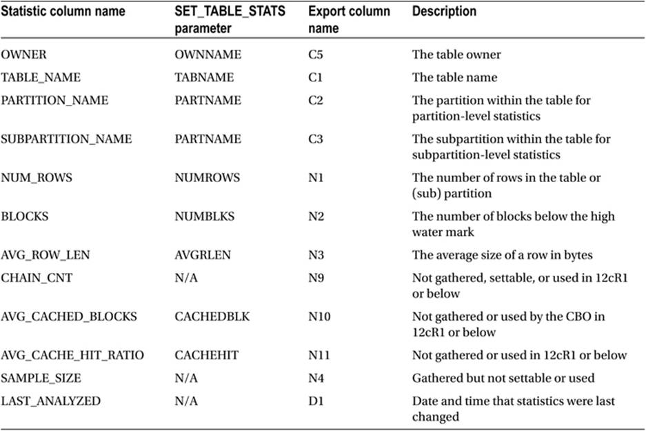
Table 9-2 shows that, as far as I can tell, the CBO only makes use of three table statistics.
· NUM_ROWS. This statistic is used in conjunction with the estimated selectivity of a row source operation to estimate the cardinality of the operation; in other words the number of rows that the operation is anticipated to return. So if NUM_ROWS is 1,000 and the selectivity is calculated as 0.1 (10%), then the estimated cardinality of the operation will be 100. The NUM_ROWS statistic is used for determining neither the number of bytes that each returned row will consume nor the cost of the operation.
· BLOCKS. This statistic is only used for full table scans and only to estimate the cost of the row source operation, in other words, how long the full table scan will take. This statistic is not used for estimating cardinality or bytes.
· AVG_ROW_LEN. This statistic is used only to estimate the number of bytes that each row returned by a row source operation will consume. In fact, only when all columns in a table are selected does the CBO have the option to use this statistic. Most of the time the column statistic AVG_COL_LEN is used for estimating the number of bytes returned by a row source operation.
The one piece of information that we are missing is the selectivity of the operation. We use column statistics to calculate selectivity, and we will come onto column statistics after looking at index statistics.
Index Statistics
Table 9-3 provides a description of each index statistic and the name by which that statistic is identified in both a statistic view and an export table. Table 9-3 also provides the name of the parameter to use in a call to DBMS_STATS.SET_INDEX_STATS.
Table 9-3. Descriptions of table statistics
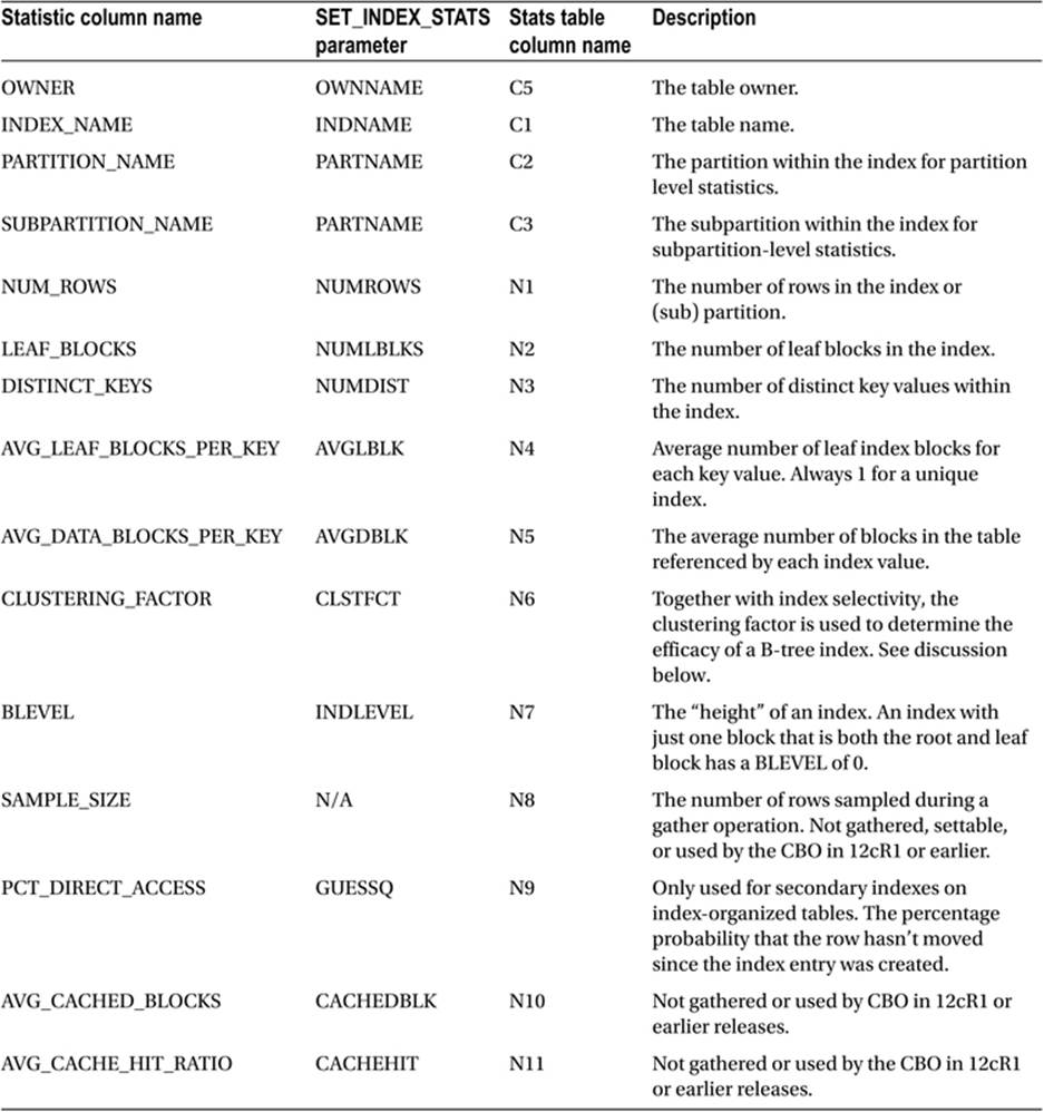
The first thing I want to say about index statistics is that they are entirely independent of table and column statistics and can be gathered solely by looking at the index without any access to the table. As an example, the statistic AVG_DATA_BLOCKS_PER_KEY, which appears to relate to the table, can be determined by looking at the ROWIDs in the index entries.
Index statistics are used to determine not only the cost, cardinalities, and bytes of an index access, but also the cost of accessing the table when the index access is a child operation of a TABLE ACCESS BY [LOCAL|GLOBAL] ROWID operation. However, before looking at how index statistics are used to cost table access, let us consider the index operation itself.
How Index Statistics are Used for Index Operations
There are a number of row source operations for accessing an index. These include INDEX RANGE SCAN, INDEX FULL SCAN, and several more. We will look at them all in Chapter 10. Once the index has been accessed, the ROWIDs returned may or may not be used to access the table itself. For now let us focus on how the CBO uses index statistics for generating estimates for the index access itself.
· NUM_ROWS. If a B-tree index is made up entirely of non-null columns then the value of NUM_ROWS for the index will exactly match the value of NUM_ROWS for the table. However, when the indexed column or columns are NULL then no entry is made for a row in a B-tree index and the value of NUM_ROWS for the index may be lower than that for the table. It turns out that sometimes the CBO estimates the cardinality of an index operation by making use of the NUM_ROWS statistic for the index, but most of the time the index statistic is ignored and the NUM_ROWS statistic for the table is used for cardinality calculations.
· LEAF_BLOCKS. This statistic is used to help determine the cost of an index operation. If the selectivity is 10% (excluding filter predicates) then the number of leaf blocks accessed is assumed to be 10% of the value of the LEAF_BLOCKS statistic.
· BLEVEL. Most index access operations involve accessing the root block of the index and working down to the leaf blocks. The BLEVEL statistic can be used directly for the estimated cost of this traversal and is added to the calculation based on LEAF_BLOCKS to arrive at the overall cost for the index operation. The costing algorithm for an INDEX FAST FULL SCAN is the one algorithm that doesn’t make use of the BLEVEL statistic, as the leaf blocks are not read by traversing the index from the root block. I will cover theINDEX FAST FULL SCAN operation in the context of other access methods in Chapter 10.
The number of bytes returned by index access operations is determined by summing the AVG_COL_LEN column statistic for all columns returned by the index operation and adding some overhead. We need to use column statistics to determine the selectivity of an index operation, just as we do for a table operation, and I will look at column statistics after explaining how index statistics are used to cost table access from an index.
How Index Statistics are Used to Cost Table Access
When a table is accessed through an index the estimated cost of that access is determined by index—not table—statistics. On the other hand, index statistics are used to determine neither the number of rows nor the number of bytes returned by the table access operation. That makes sense because the number of rows selected from a table is independent of which index, if any, is used to access the table.
Figures 9-1 and 9-2 show how difficult it is to determine the cost of accessing a table through an index.

Figure 9-1. Table blocks from a weakly clustered index

Figure 9-2. Table blocks from a strongly clustered index
Figure 9-1 shows three table blocks from an imaginary table with ten blocks that each contain 20 rows, making a total of 200 rows in the table. Let us assume that 20 rows in the table have a specific value for a specific column and that column is indexed. If these 20 rows are scattered around the table then there would be approximately two matching rows per block. I have represented this situation by the highlighted rows in Figure 9-1.
As you can see, every block in the table would need to be read to obtain these 20 rows, so a full table scan would be more efficient than an indexed access, primarily because multi-block reads could be used to access the table, rather than single block reads. Now take a look at Figure 9-2.
In this case all 20 rows that we select through the index appear in a single block, and now an indexed access would be far more efficient, as only one table block needs to be read. Notice that in both Figure 9-1 and Figure 9-2 selectivity is 10% (20 rows from 200) so knowing the selectivity isn’t sufficient for the CBO to estimate the cost of access to a table via an index. Enter the clustering factor. To calculate the cost of accessing a table through an index (as opposed to the cost of accessing the index itself) we multiply the clustering factor by the selectivity. Since strongly clustered indexes have a lower clustering factor than weakly clustered indexes, the cost of accessing the table from a strongly clustered index is lower than that for accessing the table from a weakly clustered index. Listing 9-3 demonstrates how this works in practice.
Listing 9-3. Influence of clustering factor on the cost of table access
SELECT index_name, distinct_keys, clustering_factor
FROM all_ind_statistics I
WHERE i.table_name = 'STATEMENT'
AND i.owner = SYS_CONTEXT ('USERENV', 'CURRENT_SCHEMA')
AND i.index_name IN ('STATEMENT_I_PC', 'STATEMENT_I_CC')
ORDER BY index_name DESC;
SELECT *
FROM statement t
WHERE product_category = 1;
SELECT *
FROM statement t
WHERE customer_category = 1;
SELECT /*+ index(t (customer_category)) */
*
FROM statement t
WHERE customer_category = 1;
--
-- Output of first query showing the clustering factor of the indexes
--
INDEX_NAME DISTINCT_KEYS CLUSTERING_FACTOR
STATEMENT_I_PC 10 17
STATEMENT_I_CC 50 500
--
-- Execution plans for the three queries against the STATEMENT table
--
---------------------------------------------------------------------------
| Id | Operation | Name | Cost (%CPU)|
---------------------------------------------------------------------------
| 0 | SELECT STATEMENT | | 3 (0)|
| 1 | TABLE ACCESS BY INDEX ROWID BATCHED| STATEMENT | 3 (0)|
| 2 | INDEX RANGE SCAN | STATEMENT_I_PC | 1 (0)|
---------------------------------------------------------------------------
----------------------------------------------------
| Id | Operation | Name | Cost (%CPU)|
----------------------------------------------------
| 0 | SELECT STATEMENT | | 7 (0)|
| 1 | TABLE ACCESS FULL| STATEMENT | 7 (0)|
----------------------------------------------------
---------------------------------------------------------------------------
| Id | Operation | Name | Cost (%CPU)|
---------------------------------------------------------------------------
| 0 | SELECT STATEMENT | | 11 (0)|
| 1 | TABLE ACCESS BY INDEX ROWID BATCHED| STATEMENT | 11 (0)|
| 2 | INDEX RANGE SCAN | STATEMENT_I_CC | 1 (0)|
---------------------------------------------------------------------------
I have arranged for the first 50 rows inserted into STATEMENT to have one value for PRODUCT_CATEGORY, the next 50 a second value, and so on. There are, therefore, 10 distinct values of the PRODUCT_CATEGORY, and the data is strongly clustered because all of the rows for onePRODUCT_CATEGORY will be in a small number of blocks. On the other hand, the 50 values for CUSTOMER_CATEGORY have been assigned using a MOD function, and so the rows for a specific CUSTOMER_CATEGORY are spread out over the entire table.
When we select the rows for a particular PRODUCT_CATEGORY we multiply the selectivity (1/10) by the clustering factor of the STATEMENT_I_PC index, which Listing 9-3 shows us is 17. This gives us a value of 1.7. The index access itself has a cost of 1, so the total cost of accessing the table via the index is 2.7. This is rounded to 3 for display purposes.
There are 50 different values of CUSTOMER_CATEGORY and so when we select rows for one value of CUSTOMER_CATEGORY we get only 10 rows rather than the 50 that we got when we selected rows for a particular PRODUCT_CATEGORY. Based on selectivity arguments only, you would think that if the CBO used an index to access 50 rows it would use an index to access 10 rows. However, because the selected rows for a particular CUSTOMER_CATEGORY are scattered around the table, the clustering factor is higher, and now the CBO estimates that a full table scan would be cheaper than an indexed access. The reported cost for the full table scan in Listing 9-3 is 7. When we force the use of the index with a hint, the cost of accessing the table through the index is calculated as the selectivity (1/50) multiplied by the clustering factor of theSTATEMENT_I_CC index (500). This yields a cost of 10, which is added to the cost of 1 for the index access itself to give the displayed total cost of 11. Since the estimated total cost of table access via an index is 11 and the cost of a full table scan is 5, the unhinted selection of rows for a particular CUSTOMER_CATEGORY uses a full table scan.
NESTED LOOP ACCESS VIA A MULTI-COLUMN INDEX
There is an obscure case where the cost of an index range scan is calculated in an entirely different way from how I have described above. The case involves nested loops on multi-column indexes where there is a strong correlation between the values of the indexed columns and where equality predicates exist for all indexed columns. This obscure case is identified by a low value for DISTINCT_KEYS, and the calculation involves simply adding BLEVEL and AVG_LEAF_BLOCKS_PER_KEY for the index access; the cost of the table access isAVG_DATA_BLOCKS_PER_KEY. I only mention this case to avoid leaving you with the impression that the DISTINCT_KEYS, AVG_LEAF_BLOCKS_PER_KEY, and AVG_DATA_BLOCKS_PER_KEY index statistics are unused. For more information on this obscure case seeChapter 11 of Cost-Based Oracle by Jonathan Lewis (2006).
Function-based Indexes and TIMESTAMP WITH TIME ZONE
It is possible to create an index on one or more expressions involving the columns in a table rather than just the columns themselves. Such indexes are referred to as function-based indexes. It may come as a surprise to some of you that any attempt to create an index on a column ofTIMESTAMP WITH TIME ZONE results in a function-based index! This is because columns of type TIMESTAMP WITH TIME ZONE are converted for the index in the way shown in Listing 9-4.
Listing 9-4. A function-based index involving TIMESTAMP WITH TIME ZONE
SELECT transaction_date_time
FROM statement t
WHERE transaction_date_time = TIMESTAMP '2013-01-02 12:00:00.00 -05:00';
-------------------------------------------------------------------
| Id | Operation | Name |
-------------------------------------------------------------------
| 0 | SELECT STATEMENT | |
| 1 | TABLE ACCESS BY INDEX ROWID BATCHED| STATEMENT |
| 2 | INDEX RANGE SCAN | STATEMENT_I_TRAN_DT |
-------------------------------------------------------------------
Predicate Information (identified by operation id):
---------------------------------------------------
2 - access(SYS_EXTRACT_UTC("TRANSACTION_DATE_TIME")=TIMESTAMP'
2013-01-02 17:00:00.000000000')
If you look at the filter predicate for the execution plan of the query in Listing 9-4 you will see that the predicate has changed to include a function SYS_EXTRACT_UTC that converts the TIMESTAMP WITH TIME ZONE data type to a TIMESTAMP data type indicating Universal Coordinated Time (UTC)2. The fact that the original time zone in the literal is five hours earlier than UTC is reflected in the TIMESTAMP literal in the predicate, which is shown in the execution plan. The reason that this conversion is done is because two TIMESTAMP WITH TIME ZONEvalues that involve different time zones but are actually simultaneous are considered equal. Notice that since the function-based index excludes the original time zone the table itself needs to be accessed to retrieve the time zone, even though no other column is present in the select list.
![]() Note Since all predicates involving columns of type TIMESTAMP WITH TIME ZONE are converted to use the SYS_EXTRACT_UTC function, column statistics on object columns of type TIMESTAMP WITH TIME ZONE cannot be used to determine cardinality!
Note Since all predicates involving columns of type TIMESTAMP WITH TIME ZONE are converted to use the SYS_EXTRACT_UTC function, column statistics on object columns of type TIMESTAMP WITH TIME ZONE cannot be used to determine cardinality!
Bitmap Indexes
The structure of the root block and branch blocks of a bitmap index are identical to that of a B-tree index, but the entries in the leaf blocks are bitmaps that refer to a number of rows in the table. Because of this the NUM_ROWS statistic for a bitmap index (which should be interpreted as “number of index entries” in this case) will usually be considerably less than the number of rows in the table, and for small tables will equal the number of distinct values for the column. The CLUSTERING_FACTOR is unused in a bitmap index and is set, arbitrarily, to a copy of NUM_ROWS.
Column Statistics
Finally we come to discuss column statistics. Column statistics have nothing to do with the cost of an operation and everything to do with the size of the rows returned by an operation and the cardinality of an operation. As with table and index statistics, Table 9-4 lists the individual column statistics and provides the associated identifiers in statistic views and export tables. Table 9-4 also provides the names of the parameters to DBMS_STATS.SET_COLUMN_STATS.
Table 9-4. Descriptions of table statistics
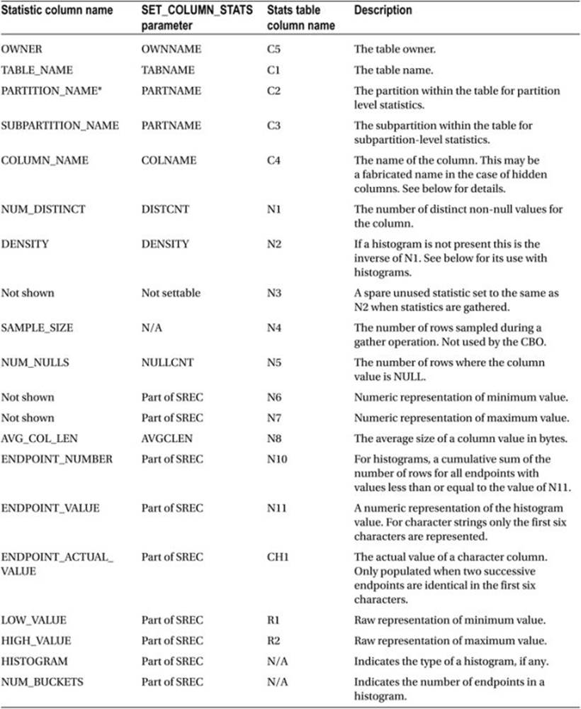
Although column statistics can be set and exported independently of table statistics, column statistics can only be gathered along with a table. The METHOD_OPT parameter to the DBMS_STATS gathering procedures controls which column statistics to gather and whether to generate histograms for these columns.
Let me first describe how column statistics are used without histograms and then explain how histograms alter things.
· NUM_DISTINCT. This statistic is sometimes used to determine selectivity. If you have an equality predicate on a column with five distinct values, the selectivity will be 1/5 or 20%. See also the DENSITY statistic.
· DENSITY.When histograms aren't in use, this statistic is the inverse of NUM_DISTINCT and is sometimes used to determine selectivity. If you have an equality predicate on a column with five distinct values, the DENSITY column will reflect the selectivity of 1/5 or 0.2.
· NUM_NULLS. This column statistic is used to help determine cardinality. The statistic is obviously invaluable when you have a predicate such as <object_column> IS NULL or <object_column> IS NOT NULL. In the latter case the number of rows selected is the value of the NUM_ROWS statistic for the object table minus the value of the NUM_NULLS statistic for the object column. The number of rows with non-null values for an object column is also the basis for cardinality calculations for equality, inequality, and range predicates.
· LOW_VALUE and HIGH_VALUE. The primary purpose of these column statistics is to handle range predicates such as TRANSACTION_DATE < DATE '2013-02-11'. Since the maximum value of TRANSACTION_DATE in the STATEMENT table created inListing 9-1 is known to be 10th January 2013, the selectivity of that predicate is estimated at 100%. I will return to the LOW_VALUE and HIGH_VALUE column statistics for a lengthier explanation in Chapter 20.
· AVG_COL_LEN. This statistic is used to determine the number of bytes returned by an operation. If, for example, you select five columns from a table then the estimate for the number of bytes returned by the operation for each row will be the sum of theAVG_COL_LEN statistics for each of those five columns plus a variable-sized overhead per row.
This explanation of column statistics seems to leave a lot out. If you pick a few SQL statements at random from a typical application and try to reproduce the CBO’s cardinality calculations based solely on the object statistics and my explanation so far you will probably succeed in very few cases. But first of all, let us look at Listing 9-5 and work through a very simple example.
Listing 9-5. Simple cardinality and bytes calculation based on column statistics
SELECT num_rows
,column_name
,num_nulls
,avg_col_len
,num_distinct
,ROUND (density, 3) density
FROM all_tab_col_statistics c, all_tab_statistics t
WHERE t.owner = SYS_CONTEXT ('USERENV', 'CURRENT_SCHEMA')
AND t.table_name = 'STATEMENT'
AND c.owner = SYS_CONTEXT ('USERENV', 'CURRENT_SCHEMA')
AND c.table_name = 'STATEMENT'
AND c.column_name IN ('TRANSACTION_DATE'
,'DESCRIPTION'
,'POSTING_DATE'
,'POSTING_DELAY');
SELECT *
FROM statement
WHERE description = 'Flight' AND posting_delay = 0;
NUM_ROWS COLUMN_NAME NUM_NULLS AVG_COL_LEN NUM_DISTINCT DENSITY
500 TRANSACTION_DATE 0 8 10 0.1
500 POSTING_DATE 0 8 12 0.083
500 POSTING_DELAY 0 3 3 0.333
500 DESCRIPTION 0 7 4 0.25
------------------------------------------------------------------
| Id | Operation | Name | Rows | Bytes | Time |
------------------------------------------------------------------
| 0 | SELECT STATEMENT | | 42 | 2310 | 00:00:01 |
| 1 | TABLE ACCESS FULL| STATEMENT | 42 | 2310 | 00:00:01 |
------------------------------------------------------------------
Listing 9-5 begins by selecting a few pertinent column statistics from our statistics views and looking at the execution plan of a simple, single table select statement on the table created in Listing 9-1.
· The first selection predicate is an equality operation on the DESCRIPTION column, and the NUM_DISTINCT column statistic for the DESCRIPTION object column is 4 (the DENSITY being 1/4).
· The second selection predicate is an equality operation on the POSTING_DELAY column, and the NUM_DISTINCT column statistic for the POSTING_DELAY object column is 3 (the DENSITY being 1/3).
· The NUM_ROWS statistic for the STATEMENT table is 500, and the NUM_NULLS statistic for the DESCRIPTION and POSTING_DELAY columns is 0, so the estimated number of rows from which we are selecting is 500.
· Given selectivities of 1/4 and 1/3 from 500 rows the estimated cardinality for the statement is 500/4/3 = 41.67, and after rounding up that is what DBMS_XPLAN displays.
That is all very well, you may say, but real-life queries have expressions and function calls in select lists and predicates. Listing 9-6 is only a little more complicated, but now the CBO’s estimates start to become a lot less scientific and a lot less accurate.
Listing 9-6. CBO calculations in the absence of column statistics
SELECT *
FROM statement
WHERE SUBSTR (description, 1, 1) = 'F';
------------------------------------------------------------------
| Id | Operation | Name | Rows | Bytes | Time |
------------------------------------------------------------------
| 0 | SELECT STATEMENT | | 5 | 275 | 00:00:01 |
| 1 | TABLE ACCESS FULL| STATEMENT | 5 | 275 | 00:00:01 |
------------------------------------------------------------------
This time our predicate involves a function call. We have no column statistic that we can use, so the CBO has to pick an arbitrary selectivity. When faced with an equality predicate and no statistics on which to base a selectivity estimate, the CBO just picks 1%! Hardcoded! So our estimated cardinality is 500/100 = 5. If you run the query you actually get 125 rows, so the estimate is out by a factor of 25.
To be fair I have given an exceptionally simplified explanation of the CBO’s cardinality-estimating algorithm, but that does not detract from the validity of the point that the CBO often makes arbitrary estimates in the absence of meaningful input data.
Histograms
The explanation of column statistics given so far means that the CBO has to treat most equality predicates involving a column name and a literal value in the same way, irrespective of the supplied value. Listing 9-7 shows how this can be problematic.
Listing 9-7. An example of a missing histogram
SELECT *
FROM statement
WHERE transaction_amount = 8;
-------------------------------------------------------------------------------
| Id | Operation | Name | Rows | Bytes | Cost (%CPU)| Time |
-------------------------------------------------------------------------------
| 0 | SELECT STATEMENT | | 2 | 106 | 8 (0)| 00:00:01 |
|* 1 | TABLE ACCESS FULL| STATEMENT | 2 | 106 | 8 (0)| 00:00:01 |
-------------------------------------------------------------------------------
There are 262 distinct values of TRANSACTION_AMOUNT in STATEMENT varying from 5 to 15200. The CBO assumes, correctly in this case, that 8 is one of those 262 values but assumes that only about 500/262 rows will have TRANSACTION_AMOUNT = 8. In actuality there are 125 rows with TRANSACTION_AMOUNT = 8. The way to improve the accuracy of the CBO’s estimate in this case is to define a histogram. Before creating the histogram I want to define what I will call a histogram specification that documents the different estimates that we want the CBO to make. I would propose the following histogram specification for TRANSACTION_AMOUNT:
For every 500 rows in STATEMENT the CBO should assume that 125 have a value of 8 for TRANSACTION_AMOUNT and the CBO should assume 2 rows for any other supplied value.
Listing 9-8 shows how we might construct a histogram to make the CBO make these assumptions.
Listing 9-8. Creating a histogram on TRANSACTION_AMOUNT
DECLARE
srec DBMS_STATS.statrec;
BEGIN
FOR r
IN (SELECT *
FROM all_tab_cols
WHERE owner = SYS_CONTEXT ('USERENV', 'CURRENT_SCHEMA')
AND table_name = 'STATEMENT'
AND column_name = 'TRANSACTION_AMOUNT')
LOOP
srec.epc := 3;
srec.bkvals := DBMS_STATS.numarray (600, 400, 600);
DBMS_STATS.prepare_column_values (srec
,DBMS_STATS.numarray (-1e7, 8, 1e7));
DBMS_STATS.set_column_stats (ownname => r.owner
,tabname => r.table_name
,colname => r.column_name
,distcnt => 3
,density => 1 / 250
,nullcnt => 0
,srec => srec
,avgclen => r.avg_col_len);
END LOOP;
END;
/
SELECT *
FROM statement
WHERE transaction_amount = 8;
------------------------------------------------------------------
| Id | Operation | Name | Rows | Bytes | Time |
------------------------------------------------------------------
| 0 | SELECT STATEMENT | | 125 | 6875 | 00:00:01 |
| 1 | TABLE ACCESS FULL| STATEMENT | 125 | 6875 | 00:00:01 |
-----------------------------------------------------------------
SELECT *
FROM statement
WHERE transaction_amount = 1640;
------------------------------------------------------------------
| Id | Operation | Name | Rows | Bytes | Time |
------------------------------------------------------------------
| 0 | SELECT STATEMENT | | 2 | 110 | 00:00:01 |
| 1 | TABLE ACCESS FULL| STATEMENT | 2 | 110 | 00:00:01 |
------------------------------------------------------------------
This PL/SQL “loop” will actually only call DBMS_STATS.SET_COLUMN_STATS once, as the query on ALL_TAB_COLS3 returns one row. The key to defining the histogram on TRANSACTION_AMOUNT is the SREC parameter that I have highlighted in bold. This structure is set up as follows:
1. Set SREC.EPC. EPC is short for End Point Count and in this case defines the number of distinct values for the object column. I recommend setting EPC to two more than the number of values for the column that the histogram specification defines. In our case the only value in our histogram specification is 8 so we set EPC to 3.
2. Set SREC.BKVALS. BKVALS is short for bucket values and in this case the list of three bucket values indicates the supposed number of rows for each endpoint. So in theory 600 rows have one value for TRANSACTION_AMOUNT, 400 rows have a second value, and 600 rows have a third value. Those three values together suggest that there are 1600 rows in the table (600+400+600=1600). In fact, the actual interpretation of these values is that for every 1600 rows in the table 600 rows have the first, as yet unspecified, value forTRANSACTION_AMOUNT, 400 rows have the second value, and 600 rows have the third value.
3. Call DBMS_STATS.PREPARE_COLUMN_VALUES to define the actual object column values for each endpoint. The first endpoint is deliberately absurdly low, the middle endpoint is the value of 8 from our histogram specification, and the last value is absurdly high. The addition of the absurdly low and absurdly high values at the beginning and end of our ordered set of values is why we set SREC.EPC to two more than the number of values in our histogram specification. We will never use the absurd values in our predicates (or they wouldn’t be absurd) so the only statistic of note is that 400 rows out of every 1600 have a value of 8. This means that when we select from 500 rows the CBO will give a cardinality estimate of 500 x 400 / 1600 = 125.
4. Call DBMS_STATS.SET_COLUMN_STATS. There are two parameters I want to draw your attention to.
· DISTCNT is set to 3. We have defined three values for our column (-1e7, 8, and 1e7) so we need to be consistent and set DISTCNT to the same value as SREC.EPC. This arrangement ensures that we get what is called a frequency histogram.
· DENSITY is set to 1/250. When a frequency histogram is defined this statistic indicates the selectivity of predicates with values not specified in the histogram. The supplied value of 1/250 in Listing 9-8 indicates that for 500 non-null rows the CBO should assume 500/250 = 2 rows match the equality predicate when a value other than the three provided appears in a predicate.
After the histogram is created we can see that the CBO provides a cardinality estimate of 125 when the TRANSACTION_AMOUNT = 8 predicate is supplied and a cardinality estimate of 2 when any other literal value is supplied in the predicate.
Creating histograms in this way is often referred to as faking histograms. I don’t like this term because there is a connotation that gathered histograms (not faked) are somehow superior. They are not. For example, when I allowed histograms to be created automatically forTRANSACTION_AMOUNT on my 12cR1 database I got a histogram with 254 endpoints. In theory, that would mean that I might get 255 different execution plans (one for each defined endpoint and one for values not specified in the histogram) for every statement involving equality predicates on TRANSACTION_AMOUNT. By manually creating a frequency histogram using a histogram specification defined with testing in mind you can limit the number of test cases. In the case of Listing 9-8 there are just two test cases for each statement: TRANSACTION_AMOUNT = 8 andTRANSACTION_AMOUNT = <anything else>.
Bear in mind the following when manually creating histograms this way:
· Manually creating a frequency histogram with absurd minimum and maximum values means that you don’t have to worry about new column values that are either higher than the previous maximum value or lower than the previous minimum. However, range predicates such as TRANSACTION_AMOUNT > 15000 may yield cardinality estimates that are far too high. If you use range predicates you may have to pick sensible minimum and maximum values.
· Don’t pick values for the srec.bkvals array that are too small or a rounding error may creep in. Don’t, for example, replace 600, 400, and 600 in Listing 9-8 with 6, 4, and 6. This will alter the results for predicates such as TRANSACTION_AMOUNT > 8.
· The CBO will get confused if the default selectivity from DENSITY is higher than the selectivity for the supplied endpoints.
· The selectivity of unspecified values of a column is only calculated using the DENSITY statistic for manually created histograms. When histograms are gathered (USER_STATS = 'NO' in ALL_TAB_COL_STATISTICS) then the selectivity of unspecified values is half of that for the lowest supplied endpoint.
· There are other types of histograms. These include height-based histograms, top frequency histograms, and hybrid histograms. Top frequency and hybrid histograms appear for the first time in 12cR1. In my experience, which may or may not be typical, the type of manually created frequency histogram that I have described here is the only one I have ever needed.
When you use one of the views listed in Table 9-1 to view histograms you may be momentarily confused. Listing 9-9 shows the histogram on TRANSACTION_AMOUNT that I created in Listing 9-8:
Listing 9-9. Displaying histogram data
SELECT table_name
,column_name
,endpoint_number
,endpoint_value
,endpoint_actual_value
FROM all_tab_histograms
WHERE owner = SYS_CONTEXT ('USERENV', 'CURRENT_SCHEMA')
AND table_name = 'STATEMENT'
AND column_name = 'TRANSACTION_AMOUNT';
TABLE_NAME COLUMN_NAME ENDPOINT_NUMBER ENDPOINT_VALUE ENDPOINT_ACTUAL_VALUE
STATEMENT TRANSACTION_AMOUNT 600 -10000000
STATEMENT TRANSACTION_AMOUNT 1000 8
STATEMENT TRANSACTION_AMOUNT 1600 10000000
The two things to be wary of are:
1. The ENDPOINT_ACTUAL_VALUE is only populated for character columns where the first six characters are shared by consecutive endpoints.
2. The ENDPOINT_NUMBER is cumulative. It represents a running sum of cardinalities up to that point.
Virtual and Hidden Columns
I have already mentioned that a function-based index creates a hidden object column and that the hidden object column can have statistics just like a regular object column. But because the column is hidden it is not returned by queries that begin SELECT * FROM. Such hidden columns are also considered to be virtual columns because they have no physical representation in the table.
Oracle database 11gR1 introduced the concept of unhidden virtual columns. These unhidden virtual columns are explicitly declared by CREATE TABLE or ALTER TABLE DDL statements rather than being implicitly declared as part of the creation of a function-based index. From the perspective of the CBO, virtual columns are treated in almost the same way, irrespective of whether they are hidden or not. Listing 9-10 shows how the CBO uses statistics on the virtual columns of the STATEMENT table created in Listing 9-1.
Listing 9-10. CBO use of statistics on virtual columns
--
-- Query 1: using an explictly declared
-- virtual column
--
SELECT *
FROM statement
WHERE posting_delay = 1;
-----------------------------------------------
| Id | Operation | Name | Rows |
-----------------------------------------------
| 0 | SELECT STATEMENT | | 167 |
|* 1 | TABLE ACCESS FULL| STATEMENT | 167 |
-----------------------------------------------
Predicate Information (identified by operation id):
---------------------------------------------------
1 - filter("POSTING_DELAY"=1)
--
-- Query 2: using an expression equivalent to
-- an explictly declared virtual column.
--
SELECT *
FROM statement
WHERE (posting_date - transaction_date) = 1;
-----------------------------------------------
| Id | Operation | Name | Rows |
-----------------------------------------------
| 0 | SELECT STATEMENT | | 167 |
|* 1 | TABLE ACCESS FULL| STATEMENT | 167 |
-----------------------------------------------
Predicate Information (identified by operation id):
---------------------------------------------------
1 - filter("STATEMENT"."POSTING_DELAY"=1)
--
-- Query 3: using an expression not identical to
-- virtual column.
--
SELECT *
FROM statement
WHERE (transaction_date - posting_date) = -1;
-----------------------------------------------
| Id | Operation | Name | Rows |
-----------------------------------------------
| 0 | SELECT STATEMENT | | 5 |
|* 1 | TABLE ACCESS FULL| STATEMENT | 5 |
-----------------------------------------------
Predicate Information (identified by operation id):
---------------------------------------------------
1 - filter("TRANSACTION_DATE"-"POSTING_DATE"=(-1))
--
-- Query 4: using a hidden column
--
SELECT /*+ full(s) */ sys_nc00010$
FROM statement s
WHERE sys_nc00010$ = TIMESTAMP '2013-01-02 17:00:00.00';
-----------------------------------------------
| Id | Operation | Name | Rows |
-----------------------------------------------
| 0 | SELECT STATEMENT | | 50 |
|* 1 | TABLE ACCESS FULL| STATEMENT | 50 |
-----------------------------------------------
Predicate Information (identified by operation id):
---------------------------------------------------
1 - filter(SYS_EXTRACT_UTC("TRANSACTION_DATE_TIME")=TIMESTAMP'
2013-01-02 17:00:00.000000000')
--
-- Query 5: using an expression equivalent to
-- a hidden column.
--
SELECT SYS_EXTRACT_UTC (transaction_date_time)
FROM statement s
WHERE SYS_EXTRACT_UTC (transaction_date_time) =
TIMESTAMP '2013-01-02 17:00:00.00';
--------------------------------------------------------
| Id | Operation | Name | Rows |
--------------------------------------------------------
| 0 | SELECT STATEMENT | | 50 |
|* 1 | INDEX RANGE SCAN| STATEMENT_I_TRAN_DT | 50 |
--------------------------------------------------------
Predicate Information (identified by operation id):
---------------------------------------------------
1 - access(SYS_EXTRACT_UTC("TRANSACTION_DATE_TIME")=TIMESTAMP'
2013-01-02 17:00:00.000000000')
--
-- Query 6: using the timestamp with time zone column
--
SELECT transaction_date_time
FROM statement s
WHERE transaction_date_time = TIMESTAMP '2013-01-02 12:00:00.00 -05:00';
---------------------------------------------------------------------------
| Id | Operation | Name | Rows |
---------------------------------------------------------------------------
| 0 | SELECT STATEMENT | | 50 |
| 1 | TABLE ACCESS BY INDEX ROWID BATCHED| STATEMENT | 50 |
|* 2 | INDEX RANGE SCAN | STATEMENT_I_TRAN_DT | 50 |
---------------------------------------------------------------------------
Predicate Information (identified by operation id):
---------------------------------------------------
2 - access(SYS_EXTRACT_UTC("TRANSACTION_DATE_TIME")=TIMESTAMP'
2013-01-02 17:00:00.000000000')
The first query in Listing 9-10 involves a predicate on an explicitly declared virtual column. The statistics for the virtual column can be used and the CBO divides the number of non-null rows by the number of distinct values for POSTING_DELAY. This is 50/3, which after rounding gives us 167. The second query uses an expression identical to the definition of the virtual column, and once again the virtual column statistics are used to yield a cardinality estimate of 167. Notice that the name of the virtual column appears in the predicate section of the execution plan of the second query. The third query uses an expression that is similar, but not identical, to the definition of the virtual column, and now the statistics on the virtual column cannot be used and the CBO has to fall back on its 1% selectivity guess.
We see similar behavior when we use predicates on the hidden column. The fourth query in Listing 9-10 somewhat unusually, but perfectly legally, references the hidden column explicitly generated for our function-based index. The CBO has been able to use the fact that there are ten distinct values of the expression in the table to estimate the cardinality as 500/10, i.e., 50. I have forced the use of a full table scan to emphasize the fact that, although the hidden column exists purely by virtue of the function-based index, the statistics can be used regardless of the access method. The fifth and sixth queries in Listing 9-10 also make use of the statistics on the hidden column. The fifth query uses the expression for the hidden column and the sixth uses the name of the TIMESTAMP WITH TIME ZONE column. Notice that in the last query the table has to be accessed to retrieve the time zone information that is missing from the index. A final observation on the last three queries is that the predicate section in the execution plan makes no reference to the hidden column name, a sensible variation of the display of filter predicates from explicitly declared virtual columns.
Extended Statistics
Like the columns created implicitly by the creation of function-based indexes, extended statistics are hidden, virtual columns. In Chapter 6 I explained the main purpose of extended statistics, namely to let the CBO understand the correlation between columns. Let me now give you an example using the STATEMENT table I created in Listing 9-1. Listing 9-11 shows two execution plans for a query, one before and one after creating extended statistics for the DESCRIPTION and AMOUNT_CATEGORY columns.
Listing 9-11. The use of multi-column extended statistics
--
-- Query and associated execution plan without extended statistics
--
SELECT *
FROM statement t
WHERE transaction_date = DATE '2013-01-02'
AND posting_date = DATE '2013-01-02';
----------------------------------------------------------
| Id | Operation | Name | Rows | Time |
----------------------------------------------------------
| 0 | SELECT STATEMENT | | 4 | 00:00:01 |
|* 1 | TABLE ACCESS FULL| STATEMENT | 4 | 00:00:01 |
----------------------------------------------------------
--
-- Now we gather extended statistics for the two columns
--
DECLARE
extension_name all_tab_col_statistics.column_name%TYPE;
BEGIN
extension_name :=
DBMS_STATS.create_extended_stats (
ownname => SYS_CONTEXT ('USERENV', 'CURRENT_SCHEMA')
,tabname => 'STATEMENT'
,extension => '(TRANSACTION_DATE,POSTING_DATE)');
DBMS_STATS.gather_table_stats (
ownname => SYS_CONTEXT ('USERENV', 'CURRENT_SCHEMA')
,tabname => 'STATEMENT'
,partname => NULL
,GRANULARITY => 'GLOBAL'
,method_opt => 'FOR ALL COLUMNS SIZE 1'
,cascade => FALSE);
END;
/
--
-- Now let us look at the new execution plan for the query
--
----------------------------------------------------------
| Id | Operation | Name | Rows | Time |
----------------------------------------------------------
| 0 | SELECT STATEMENT | | 17 | 00:00:01 |
|* 1 | TABLE ACCESS FULL| STATEMENT | 17 | 00:00:01 |
----------------------------------------------------------
The query in Listing 9-11 includes predicates on the TRANSACTION_DATE and POSTING_DATE columns. There are 10 values for TRANSACTION_DATE and 12 values for POSTING_DATE, and so without the extended statistics the CBO assumes that the query will return 500/10/12 rows, which is about 4. In fact, there are only 30 different combinations of TRANSACTION_DATE and POSTING_DATE, and after the extended statistics are gathered the execution plan for our query shows a cardinality of 17, which is the rounded result of 500/30.
![]() Note I might have created the TRANSACTION_DATE column as a virtual column derived by the expression TRUNC (TRANSACTION_DATE_TIME). However, extended statistics, such as that defined in Listing 9-11, cannot be based on virtual columns.
Note I might have created the TRANSACTION_DATE column as a virtual column derived by the expression TRUNC (TRANSACTION_DATE_TIME). However, extended statistics, such as that defined in Listing 9-11, cannot be based on virtual columns.
I have said that with respect to cardinality estimates we shouldn’t be overly concerned by errors of factors of 2 or 3, and the difference between 17 and 4 isn’t much more than that. However, it is quite common to have several predicates on a number of correlated columns, and the cumulative effect of these sorts of cardinality errors can be disastrous.
![]() Note In Chapter 6, I mentioned that when you begin to analyze the performance of a new application or a new major release of an existing application it is a good idea to look for ways to improve the execution plans of large numbers of statements. Extended statistics are a prime example of this sort of change: if you set up extended statistics properly, the CBO may improve execution plans for a large number of statements.
Note In Chapter 6, I mentioned that when you begin to analyze the performance of a new application or a new major release of an existing application it is a good idea to look for ways to improve the execution plans of large numbers of statements. Extended statistics are a prime example of this sort of change: if you set up extended statistics properly, the CBO may improve execution plans for a large number of statements.
There is a second variety of extended statistics that can be useful. This type of extension is just like the hidden virtual column that you get with a function-based index but without the index itself. Listing 9-12 shows an example.
Listing 9-12. Extended statistics for an expression
SELECT *
FROM statement
WHERE CASE
WHEN description <> 'Flight' AND transaction_amount > 100
THEN
'HIGH'
END = 'HIGH';
----------------------------------------------------------
| Id | Operation | Name | Rows | Time |
----------------------------------------------------------
| 0 | SELECT STATEMENT | | 5 | 00:00:01 |
|* 1 | TABLE ACCESS FULL| STATEMENT | 5 | 00:00:01 |
----------------------------------------------------------
Predicate Information (identified by operation id):
---------------------------------------------------
1 - filter(CASE WHEN ("DESCRIPTION"<>'Flight' AND
"TRANSACTION_AMOUNT">100) THEN 'HIGH' END ='HIGH')
DECLARE
extension_name all_tab_cols.column_name%TYPE;
BEGIN
extension_name :=
DBMS_STATS.create_extended_stats (
ownname => SYS_CONTEXT ('USERENV', 'CURRENT_SCHEMA')
,tabname => 'STATEMENT'
,extension => q'[(CASE WHEN DESCRIPTION <> 'Flight'
AND TRANSACTION_AMOUNT > 100
THEN 'HIGH' END)]');
DBMS_STATS.gather_table_stats (
ownname => SYS_CONTEXT ('USERENV', 'CURRENT_SCHEMA')
,tabname => 'STATEMENT'
,partname => NULL
,method_opt => 'FOR ALL COLUMNS SIZE 1'
,cascade => FALSE);
END;
/
----------------------------------------------------------
| Id | Operation | Name | Rows | Time |
----------------------------------------------------------
| 0 | SELECT STATEMENT | | 105 | 00:00:01 |
|* 1 | TABLE ACCESS FULL| STATEMENT | 105 | 00:00:01 |
----------------------------------------------------------
Predicate Information (identified by operation id):
---------------------------------------------------
1 - filter(CASE WHEN ("DESCRIPTION"<>'Flight' AND
"TRANSACTION_AMOUNT">100) THEN 'HIGH' END ='HIGH')
The query in Listing 9-12 lists all transactions with AMOUNT > 100 that aren’t flights. The query has had to be constructed in a special way so that we can take advantage of extended statistics. Before the creation of the extended statistic the estimated cardinality is 5 based on our good old 1% estimate. After the creation of an extended statistic on our carefully constructed expression, and the subsequent gathering of statistics on the table, we can see that the CBO has been able to accurately estimate the number of rows that would be returned from the query at 105.
Viewing Information on Virtual and Hidden Columns
As we have seen, the statistics for hidden and virtual columns are the same as for regular columns; the CBO uses these statistics in similar ways. However, there are two more things to be said about hidden and virtual columns. I want to explain how extended statistics are exported, but first let us look at how to examine information on hidden and virtual columns in the data dictionary.
Data Dictionary Views for Hidden and Virtual Columns
Hidden columns are not displayed by the view ALL_TAB_COLUMNS and only appear in ALL_TAB_COL_STATISTICS if statistics exist on the hidden columns. There are two views that display information on hidden columns regardless of whether they have statistics or not:
· ALL_TAB_COLS displays similar information as ALL_TAB_COLUMNS but includes hidden columns. The ALL_TAB_COLS statistic view includes two statistic columns—VIRTUAL_COLUMN and HIDDEN_COLUMN—that indicate if the object column is virtual or hidden, respectively.
· ALL_STAT_EXTENSIONS lists information about all virtual columns, including hidden virtual columns, whether they are associated with function-based indexes; unhidden, explicitly declared virtual columns; or hidden columns associated with extended statistics.ALL_STAT_EXTENSIONS includes a column—EXTENSION—with a data type of CLOB that defines the expression upon which the virtual column is based.
Exporting Extended Statistics
With the exception of extended statistics, hidden and virtual columns are exported and imported in precisely the same way as regular columns. However, there is an additional row in an export table for each extended statistic.
You cannot import statistics for a hidden column associated with a function-based index without creating the function-based index first using a CREATE INDEX statement. You cannot import statistics for an explicitly declared virtual column without declaring the column first using aCREATE TABLE or ALTER TABLE statement. The DDL statements that create function-based indexes and explicitly declared virtual columns cause the expressions on which the virtual column is based to be stored in the data dictionary.
On the other hand, you can import extended statistics without first calling DBMS_STATS.CREATE_EXTENDED_STATS; the import operation implicitly creates the hidden virtual column. This implicit creation of virtual columns that occurs when statistics are imported means that the export table needs to contain information about the expression on which the virtual column is based. This information is held in an extra row in the export table that has a TYPE of E, and the expression is stored in the export column CL1 that is of type CLOB. Listing 9-13 shows how extended statistics can be exported and imported.
Listing 9-13. Exporting and importing extended statistcs
TRUNCATE TABLE ch9_stats;
BEGIN
DBMS_STATS.export_table_stats (
ownname => SYS_CONTEXT ('USERENV', 'CURRENT_SCHEMA')
,tabname => 'STATEMENT'
,statown => SYS_CONTEXT ('USERENV', 'CURRENT_SCHEMA')
,stattab => 'CH9_STATS');
DBMS_STATS.drop_extended_stats (
ownname => SYS_CONTEXT ('USERENV', 'CURRENT_SCHEMA')
,tabname => 'STATEMENT'
,extension => '(TRANSACTION_DATE,POSTING_DATE)');
DBMS_STATS.drop_extended_stats (
ownname => SYS_CONTEXT ('USERENV', 'CURRENT_SCHEMA')
,tabname => 'STATEMENT'
,extension => q'[(CASE WHEN DESCRIPTION <> 'Flight'
AND TRANSACTION_AMOUNT > 100
THEN 'HIGH' END)]');
DBMS_STATS.delete_table_stats (
ownname => SYS_CONTEXT ('USERENV', 'CURRENT_SCHEMA')
,tabname => 'STATEMENT');
END;
/
SELECT c1, SUBSTR (c4, 1,10) c4, DBMS_LOB.SUBSTR (cl1,60,1) cl1
FROM ch9_stats
WHERE TYPE = 'E';
-- Output from select statement
C1 C4 CL1
STATEMENT SYS_STU557 SYS_OP_COMBINED_HASH("TRANSACTION_DATE","POSTING_DATE")
STATEMENT SYS_STUN6S CASE WHEN ("DESCRIPTION"<>'Flight' AND "TRANSACTION_AMOUNT"
SELECT extension_name
FROM all_stat_extensions
WHERE owner = SYS_CONTEXT ('USERENV', 'CURRENT_SCHEMA')
AND table_name = 'STATEMENT'
ORDER BY extension_name;
-- Output from select statement
EXTENSION_NAME
AMOUNT_CATEGORY
POSTING_DELAY
SYS_NC00010$
BEGIN
DBMS_STATS.import_table_stats (
ownname => SYS_CONTEXT ('USERENV', 'CURRENT_SCHEMA')
,tabname => 'STATEMENT'
,statown => SYS_CONTEXT ('USERENV', 'CURRENT_SCHEMA')
,stattab => 'CH9_STATS');
END;
/
SELECT extension_name
FROM all_stat_extensions
WHERE owner = SYS_CONTEXT ('USERENV', 'CURRENT_SCHEMA')
AND table_name = 'STATEMENT'
ORDER BY extension_name;
-- Output from select statement
EXTENSION_NAME
AMOUNT_CATEGORY
POSTING_DELAY
SYS_NC00010$
SYS_STU557IEAHGZ6B4RPUZEQ_SX#6
SYS_STUN6S71CM11RD1VMYVLKR9$GJ
Listing 9-14 exports the object statistics for STATEMENT into a freshly truncated export table and then drops both extended statistics with the DBMS_STATS.DROP_EXTENDED_STATISTICS procedure. The remaining statistics are dropped as well just for good measure.
A query against the export table shows that the specification of the extended statistics expressions has been saved. Notice the use of the SYS_OP_COMBINED_HASH function for the multi-column statistic. Once the extended statistics are dropped we can see that they are no longer visible in the output of a query against ALL_STAT_EXTENSIONS.
Once we import the statistics we can see the extended statistics reappear in ALL_STAT_EXTENSIONS.
Statistics Descriptions Wrap-up
I have explained what the statistics associated with tables, indexes, and columns are and how they are used by the CBO for optimization. I have also explained the major different types of hidden and virtual columns that can be created and used by the CBO. What I have yet to do is to explain the various different levels of statistics that can be used on partitioned tables. Let us get into that now.
Statistics and Partitions
The partitioning option is a separately licensed feature of Oracle Database Enterprise Edition. With this option you are able to partition your tables and indexes and enjoy a number of performance and administrative benefits. I will briefly look at the performance benefits of partitioning inChapter 15, but for the moment I want to focus on the statistics associated with partitioned tables.
As I mentioned in the introduction to this chapter, when the partitioning option is used, table, index, and column statistics can all be maintained at the global, partition, and, in the case of composite partitioned tables, subpartition level. The statistics associated with a table or index partition are precisely the same as those at the global level. For example, the AVG_ROW_LEN statistic for a table partition indicates the average size of a row in the table partition. The BLEVEL statistic of an index partition indicates how many blocks have to be visited on the way from the index partition’s root block to a leaf block within the index partition. The NUM_NULLS statistic for an object column defined at the partition level indicates the number of rows within the specified table partition where the object column is NULL.
In this section I want to clear up some confusion around how and when the CBO uses partition- and subpartition-level statistics and when global statistics are used. I also want to clearly explain the difference between the use of partition-level statistics by the CBO and partition eliminationby the runtime engine.
Before getting into these topics, however, I need to explain how partition-level statistics are obtained. Setting, exporting, and importing statistics for a particular partition or subpartition is the same as doing so for the table or index as a whole, barring the specification of the partition or subpartition name; I won’t revisit these topics. However, there are a couple of complications regarding gathering statistics at the partition or subpartition level, which I will cover now.
The relationship between table statistics and partition-level statistics can be extended to the relationship between partition-level statistics and subpartition-level statistics. To be concise, I will ignore composite partitioned tables and subpartition-level statistics for most of the rest of this section.
Gathering Statistics on Partitioned Tables
When we call routines such as DBMS_STATS.GATHER_TABLE_STATS providing the name of a partitioned table as a parameter, we have the opportunity to specify a value for the GRANULARITY parameter. For partitioned tables the default value for GRANULARITY is ALL, which means that both global and partition-level statistics are gathered.
You might think that by scanning the data in each partition of a partitioned table it would be possible to construct global and partition-level statistics at the same time. This is not the default behavior.
If you specify ALL for the GRANULARITY parameter of DBMS_STATS.GATHER_TABLE_STATS and NULL for the PARTNAME parameter, what actually happens by default is that all the partitions are scanned twice. One scan is used to obtain the global statistics and another to obtain the partition-level statistics. So if your table has five partitions you will have a total of ten partition scans.
If you specify ALL for the GRANULARITY parameter of DBMS_STATS.GATHER_TABLE_STATS and the name of a specific partition for the PARTNAME parameter, then partition-level statistics are gathered only for the specified partition, but all partitions are scanned to gather global statistics. Thus, if your table has five partitions you have a total of six partition scans.
Many users like to gather partition-level statistics when data is loaded into a previously empty partition and the overhead of scanning all partitions to update global statistics is unacceptable. As a consequence, it is normal for calls to DBMS_STATS.GATHER_TABLE_STATS to specify a value of PARTITION for the GRANULARITY parameter when gathering statistics on a single partition. This setting means that only one scan is made on the specified partition and no scans are made on any other partition. Fortunately, the negative impact of this shortcut is far less than you might think. Listing 9-14 shows what happens to global statistics when they aren’t explicitly gathered.
Listing 9-14. Gathering statistics with GRANULARITY set to PARTITION
CREATE /*+ NO_GATHER_OPTIMIZER_STATISTICS */TABLE statement_part
PARTITION BY RANGE
(transaction_date)
(
PARTITION p1 VALUES LESS THAN (DATE '2013-01-05')
,PARTITION p2 VALUES LESS THAN (maxvalue))
AS
SELECT * FROM statement;
BEGIN
DBMS_STATS.gather_table_stats (
ownname => SYS_CONTEXT ('USERENV', 'CURRENT_SCHEMA')
,tabname => 'STATEMENT_PART'
,partname => 'P1'
,GRANULARITY => 'PARTITION'
,method_opt => 'FOR ALL COLUMNS SIZE 1');
DBMS_STATS.gather_table_stats (
ownname => SYS_CONTEXT ('USERENV', 'CURRENT_SCHEMA')
,tabname => 'STATEMENT_PART'
,partname => 'P2'
,GRANULARITY => 'PARTITION'
,method_opt => 'FOR ALL COLUMNS SIZE 1');
END;
/
SELECT a.num_rows p1_rows
,a.global_stats p1_global_stats
,b.num_rows p2_rows
,b.global_stats p2_global_stats
,c.num_rows tab_rows
,c.global_stats tab_global_stats
FROM all_tab_statistics a
FULL JOIN all_tab_statistics b USING (owner, table_name)
FULL JOIN all_tab_statistics c USING (owner, table_name)
WHERE owner = SYS_CONTEXT ('USERENV', 'CURRENT_SCHEMA')
AND table_name = 'STATEMENT_PART'
AND a.partition_name = 'P1'
AND b.partition_name = 'P2'
AND c.partition_name IS NULL;
P1_ROWS P1_GLOBAL_STATS P2_ROWS P2_GLOBAL_STATS TAB_ROWS TAB_GLOBAL_STATS
200 YES 300 YES 500 NO
Listing 9-14 creates a table STATEMENT_PART that has the same content as STATEMENT, but all virtual columns have become real and the table is partitioned by range using the TRANSACTION_DATE column. Two partitions are created; they are named, somewhat unimaginatively, P1and P2. I have specified the NO_GATHER_OPTIMIZER_STATISTICS hint so that on 12cR1 and later global statistics are not gathered automatically.
Once STATEMENT_PART is created and populated, statistics are gathered on the two partitions—P1 and P2—individually. Listing 9-14 then proceeds to look at the NUM_ROWS and GLOBAL_STATS statistic columns for the two partitions and for the table as a whole. We can see that there are apparently 200 rows in partition P1 and 300 rows in P2. However, in apparent contradiction to my explanation of the GRANULARITY parameter above, there are global statistics for the table as a whole because NUM_ROWS in ALL_TAB_STATISTICS has been set to 500!
The key to understanding what has happened is to look at the value of the column named GLOBAL_STATS. Now, I was utterly confused by this column for many years. I used to think that GLOBAL_STATS, which is set to YES or NO, had something to do with whether the statistics were global statistics or not. I hope you can sympathize with my mistake. If I had read the Reference manual properly I would have seen the following:
GLOBAL_STATS VARCHAR2 (3) Indicates whether statistics were calculated without merging underlying partitions (YES) or not (NO)
It was only a short while ago that I was put out of my misery by Doug Burns (http://oracledoug.com/index.html), who explained the concept properly in a conference presentation. You see, once statistics are available for all partitions in a table or index, these partition-level statistics can be merged to determine the global statistics. In this case the numbers 200 from P1 and 300 from P2 are just added up to get 500 for STATEMENT_PART as a whole.
This method of merging partition-level statistics might seem to render the need for gathering global statistics unnecessary. However, this isn’t quite true. Listing 9-15 shows the one issue that relates to merging partition-level statistics.
Listing 9-15. NUM_DISTINCT calculations when merging partition-level statistics
SELECT column_name
,a.num_distinct p1_distinct
,b.num_distinct p2_distinct
,c.num_distinct tab_distinct
FROM all_part_col_statistics a
FULL JOIN all_part_col_statistics b
USING (owner, table_name, column_name)
FULL JOIN all_tab_col_statistics c
USING (owner, table_name, column_name)
WHERE owner = SYS_CONTEXT ('USERENV', 'CURRENT_SCHEMA')
AND table_name = 'STATEMENT_PART'
AND a.partition_name = 'P1'
AND b.partition_name = 'P2';
COLUMN_NAME P1_DISTINCT P2_DISTINCT TAB_DISTINCT
CUSTOMER_CATEGORY 50 50 50
PRODUCT_CATEGORY 4 6 10
AMOUNT_CATEGORY 3 3 3
TRANSACTION_AMOUNT 112 166 166
DESCRIPTION 4 4 4
POSTING_DELAY 3 3 3
POSTING_DATE 6 8 8
TRANSACTION_DATE 4 6 10
TRANSACTION_DATE_TIME 4 6 10
Listing 9-15 queries the NUM_DISTINCT statistic columns for partitions P1 and P2 and for the table as a whole. We can see that there are four distinct values of TRANSACTION_DATE_TIME in P1 and six distinct values in P2. The DBMS_STATS package had correctly determined that there are a total of ten distinct values of TRANSACTION_DATE_TIME in the table as a whole because the maximum value of TRANSACTION_DATE_TIME in P1 is lower than the minimum value in P2. On the other hand, DBMS_STATS sees that there are six distinct values ofPOSTING_DATE in P1 and eight in P2, but it has no way of knowing whether the number of distinct values of POSTING_DATE in the table as a whole is 8, 14, or something in between. The confusion arises because the maximum value of POSTING_DATE in P1 is greater than the minimum value in P2. The actual number of distinct values of POSTING_DATE in STATEMENT_PART is 12. DBMS_STATS always takes the minimum possible value in these circumstances.
Oracle database 11gR1 introduced a fancy new feature that allows us to get accurate, or almost accurate, global column statistics by merging partition column statistics. Listing 9-16 shows us how we can do this.
Listing 9-16. Incremental gathering of global statistics
BEGIN
DBMS_STATS.set_table_prefs(
ownname => SYS_CONTEXT ('USERENV', 'CURRENT_SCHEMA')
,tabname => 'STATEMENT_PART'
,pname => 'INCREMENTAL'
,pvalue => 'TRUE');
END;
/
BEGIN
DBMS_STATS.gather_table_stats (
ownname => SYS_CONTEXT ('USERENV', 'CURRENT_SCHEMA')
,tabname => 'STATEMENT_PART'
,partname => 'P1'
,GRANULARITY => 'APPROX_GLOBAL AND PARTITION'
,method_opt => 'FOR ALL COLUMNS SIZE 1');
DBMS_STATS.gather_table_stats (
ownname => SYS_CONTEXT ('USERENV', 'CURRENT_SCHEMA')
,tabname => 'STATEMENT_PART'
,partname => 'P2'
,granularity => 'APPROX_GLOBAL AND PARTITION'
,method_opt => 'FOR ALL COLUMNS SIZE 1');
END;
/
SELECT column_name
,a.num_distinct p1_distinct
,b.num_distinct p2_distinct
,c.num_distinct tab_distinct
FROM all_part_col_statistics a
FULL JOIN all_part_col_statistics b
USING (owner, table_name, column_name)
FULL JOIN all_tab_col_statistics c
USING (owner, table_name, column_name)
WHERE owner = SYS_CONTEXT ('USERENV', 'CURRENT_SCHEMA')
AND table_name = 'STATEMENT_PART'
AND a.partition_name = 'P1'
AND b.partition_name = 'P2';
COLUMN_NAME P1_DISTINCT P2_DISTINCT TAB_DISTINCT
CUSTOMER_CATEGORY 50 50 50
PRODUCT_CATEGORY 4 6 10
AMOUNT_CATEGORY 3 3 3
TRANSACTION_AMOUNT 112 166 262
DESCRIPTION 4 4 4
POSTING_DELAY 3 3 3
POSTING_DATE 6 8 12
TRANSACTION_DATE 4 6 10
TRANSACTION_DATE_TIME 4 6 10
Listing 9-16 uses the DBMS_STATS.SET_TABLE_PREFS procedure to set up what are called synopses for partitions. Statistics for partitions P1 and P2 are then gathered with the GRANULARITY of “APPROX_GLOBAL AND PARTITION,” and at that point the calculation for the global NUM_DISTINCT statistics has been corrected. In particular, notice that the number of distinct values of POSTING_DATE for the table as a whole is now 12.
![]() Note There are a number of other preferences that you can set with DBMS_STATS.SET_DATABASE_PREFS, DBMS_STATS.SET_SCHEMA_PREFS, and DBMS_STATS.SET_TABLE_PREFS. I will explain shortly why you should leave most of them alone.
Note There are a number of other preferences that you can set with DBMS_STATS.SET_DATABASE_PREFS, DBMS_STATS.SET_SCHEMA_PREFS, and DBMS_STATS.SET_TABLE_PREFS. I will explain shortly why you should leave most of them alone.
For columns with a small number of distinct values, a synopsis is essentially just a list of those distinct values, and statistics merging is 100% accurate, as in Listing 9-16. When there are a large number of distinct values some fancy hashing occurs possibly, resulting in some slight inaccuracies in the merged statistics. In most cases the use of incrementally maintained global statistics will reduce the total amount of time needed to gather statistics, and the global statistics that result will be perfectly usable. On the other hand, synopses take up space and increase the time that it takes to gather partition-level statistics. Many users still like to gather partition-level statistics as quickly as possible (without synopses) during the week and gather global statistics on the weekend when the system is less busy.
Here are a few points to wrap up the topic of gathering partition-level statistics:
· When the INCREMENTAL preference is used and APPROX_GLOBAL AND PARTITION is specified for GRANULARITY, then GLOBAL_STATS=YES for the table/index as a whole despite the fact that the statistics have actually been obtained by merging partition-level statistics.
· When GLOBAL_STATS=NO for a partition it means that statistics for the partition have been merged from subpartition-level statistics. GLOBAL_STATS has no meaning for subpartition-level statistics.
· GLOBAL_STATS and USER_STATS are both set to YES by DBMS_STATS.SET_xxx_STATS procedures.
· Updating global statistics by merging partition statistics doesn’t always happen. For example, merging doesn’t happen when there are existing statistics for the table/index as a whole and those statistics have GLOBAL_STATS=YES. It doesn’t matter how old these unmerged statistics are, they will never be updated by statistics merged from partition-level statistics unless the APPROX_GLOBAL AND PARTITION GRANULARITY parameter value is used when gathering partition-level statistics. There are, apparently, other undocumented scenarios where merging of partition-level statistics into global statistics will not occur.
· If the INCREMENTAL preference has been set to TRUE with a call to DBMS_STATS.SET_TABLE_PREFS, then gathering statistics for the table as a whole, specifying a value of GLOBAL for GRANULARITY, will actually gather partition-level statistics and merge them. So GLOBAL and ALL appear to be equivalent values for GRANULARITY in such a case.
How the CBO Uses Partition-level Statistics
Now that we have covered what partition-level statistics are and how we obtain them, it is time to look at how the CBO uses them. It seems that a lot of people get the use of partition-level statistics by the CBO confused with the concept of partition elimination by the runtime engine. Listings 9-17 through 9-20 should help clear things up.
Listing 9-17. Partition elimination by the runtime engine and partition statistics by the CBO
SELECT *
FROM statement_part
WHERE transaction_date = DATE '2013-01-01'
AND posting_date = DATE '2013-01-01';
--------------------------------------------------------------------------------------------
| Id | Operation | Name | Rows | Bytes | Time | Pstart| Pstop |
--------------------------------------------------------------------------------------------
| 0 | SELECT STATEMENT | | 8 | 424 | 00:00:01 | | |
| 1 | PARTITION RANGE SINGLE| | 8 | 424 | 00:00:01 | 1 | 1 |
|* 2 | TABLE ACCESS FULL | STATEMENT_PART | 8 | 424 | 00:00:01 | 1 | 1 |
--------------------------------------------------------------------------------------------
SELECT *
FROM statement_part
WHERE transaction_date = DATE '2013-01-06'
AND posting_date = DATE '2013-01-06';
--------------------------------------------------------------------------------------------
| Id | Operation | Name | Rows | Bytes | Time | Pstart| Pstop |
--------------------------------------------------------------------------------------------
| 0 | SELECT STATEMENT | | 6 | 324 | 00:00:01 | | |
| 1 | PARTITION RANGE SINGLE| | 6 | 324 | 00:00:01 | 2 | 2 |
|* 2 | TABLE ACCESS FULL | STATEMENT_PART | 6 | 324 | 00:00:01 | 2 | 2 |
--------------------------------------------------------------------------------------------
Because of the predicate on TRANSACTION_DATE in the queries in Listing 9-17, the CBO knows precisely which partition will be accessed. In the first query, the CBO knows that only the first partition, P1, will be referenced. The CBO tells us this by listing the number 1 in thePSTART (partition start) and PSTOP (partition stop) columns in the operation table. Accordingly, the CBO can use the partition-level statistics for P1 in its calculations. The partition-level statistics for P1 indicate the following:
· There are 300 rows in partition P1.
· There are six different values for TRANSACTION_DATE and six different values for POSTING_DATE in partition P1.
· So that gives us an estimated cardinality of 300/6/6 = 8.33 rows (rounded to 8).
The second query in Listing 9-17 is known by the CBO to use the second partition, so the statistics for P2 are used:
· There are 200 rows in partition P2.
· There are four different values for TRANSACTION_DATE and eight different values for POSTING_DATE in partition P2.
· So that gives us an estimated cardinality of 200/4/8 = 6.25 rows (rounded to 6).
The different cardinality estimates for the two queries is clear evidence that the CBO has used partition-level statistics in its calculations. Listing 9-18 shows us a third query that differs only slightly from those in Listing 9-17, but that difference is crucial.
Listing 9-18. Partition elimination by the runtime engine and use of global statistics by the CBO
SELECT *
FROM statement_part
WHERE transaction_date = (SELECT DATE '2013-01-01' FROM DUAL)
AND posting_date = DATE '2013-01-01';
--------------------------------------------------------------------------------------------
| Id | Operation | Name | Rows | Bytes | Time | Pstart| Pstop |
--------------------------------------------------------------------------------------------
| 0 | SELECT STATEMENT | | 4 | 220 | 00:00:01 | | |
| 1 | PARTITION RANGE SINGLE| | 4 | 220 | 00:00:01 | KEY | KEY |
|* 2 | TABLE ACCESS FULL | STATEMENT_PART | 4 | 220 | 00:00:01 | KEY | KEY |
| 3 | FAST DUAL | | 1 | | 00:00:01 | | |
--------------------------------------------------------------------------------------------
Listing 9-18 doesn’t use a literal for the TRANSACTION_DATE value. It uses an expression. That simple change means that the CBO loses track of which partition will be referenced, a fact that is made clear by the use of the word “KEY" in the PSTART and PSTOP columns of the operation table. As a consequence of this lack of certainty the CBO falls back on global statistics, as follows:
· There are 500 rows in STATEMENT_PART, according to the global statistics.
· There are 10 different values for TRANSACTION_DATE in STATEMENT_PART, according to the global statistics.
· There are 12 different values for POSTING_DATE in STATEMENT_PART, according to the global statistics.
· So that gives us an estimated cardinality of 500/10/12 = 4.17 rows (rounded to 4).
I want to be absolutely clear about something: the CBO does know that only a single partition will be referenced. That is why it was able to specify the PARTITION RANGE SINGLE operation. The runtime engine will be able to restrict its access to one partition. However, whichpartition the runtime engine will use remains unknown until the little subquery is actually run. So even though only a single partition is accessed at runtime the CBO needs to use global statistics to estimate the cardinality, because the CBO doesn’t know which set of partition-level statistics to use.
The last two listings have covered queries that access just a single partition. Listing 9-19 shows a query that references multiple partitions:
Listing 9-19. Use of global statistics when multiple partitions are referenced
SELECT *
FROM statement_part
WHERE transaction_date IN (DATE '2013-01-04', DATE '2013-01-05')
AND posting_date = DATE '2013-01-05';
--------------------------------------------------------------------------------------------
| Id | Operation | Name | Rows | Bytes | Time | Pstart| Pstop |
--------------------------------------------------------------------------------------------
| 0 | SELECT STATEMENT | | 8 | 440 | 00:00:01 | | |
| 1 | PARTITION RANGE INLIST| | 8 | 440 | 00:00:01 |KEY(I) |KEY(I) |
|* 2 | TABLE ACCESS FULL | STATEMENT_PART | 8 | 440 | 00:00:01 |KEY(I) |KEY(I) |
--------------------------------------------------------------------------------------------
Listing 9-19 references two values of TRANSACTION_DATE in different partitions. The CBO knows which partitions are used for each value of the inlist, so theoretically the CBO could use the statistics for partition P1 to estimate the number of rows where TRANSACTION_DATE is 4th January and the statistics for P2 to estimate the number of rows where TRANSACTION_DATE is 5th January. This would have yielded a cardinality estimate of 14 (8+6). However, the CBO is designed to use only one set of statistics at a time and so uses the global statistics for both dates. Hence the cardinality estimate of 8 (4+4). Notice the PSTART and PSTOP columns in the operation table have a value of KEY (I), indicating the presence of an inlist.
There is one final reason why global statistics might be used, and that is because partition-level statistics do not exist! For completeness, Listing 9-20 demonstrates this case.
Listing 9-20. Deleting partition-level statistics
BEGIN
DBMS_STATS.delete_table_stats (
ownname => SYS_CONTEXT ('USERENV', 'CURRENT_SCHEMA')
,tabname => 'STATEMENT_PART'
,partname => 'P1');
END;
/
SELECT *
FROM statement_part
WHERE transaction_date = DATE '2013-01-01'
AND posting_date = DATE '2013-01-01';
--------------------------------------------------------------------------------------------
| Id | Operation | Name | Rows | Bytes | Time | Pstart| Pstop |
--------------------------------------------------------------------------------------------
| 0 | SELECT STATEMENT | | 4 | 220 | 00:00:01 | | |
| 1 | PARTITION RANGE SINGLE| | 4 | 220 | 00:00:01 | 1 | 1 |
|* 2 | TABLE ACCESS FULL | STATEMENT_PART | 4 | 220 | 00:00:01 | 1 | 1 |
--------------------------------------------------------------------------------------------
Listing 9-20 shows an execution plan for the same query as that in Listing 9-17 except that the partition-level statistics are deleted. We can see that the CBO still knows the specific partition to be referenced, but the cardinality estimate of 4 shows that we have used global statistics as the basis for estimation in the same way as in Listing 9-18.
Why We Need Partition-level Statistics
Now that I have explained what partition-level statistics are, I can address the question of why partition-level statistics are needed in the first place. To be clear: partition-level statistics aren’t always required. The CBO can often work out fairly reasonable plans perfectly well with just global statistics. There are three main reasons why people bother with partition level statistics:
· The amount of data varies substantially from one partition to the next and so different execution plans may be needed when querying different partitions.
· It takes too long to gather global statistics.
· Partition-level statistics appear to result in the CBO picking better performing plans.
Let us look at each of these reasons in turn.
Skew in Partition Size
When the partitioning option is used to facilitate what the VLDB and Partitioning Guide calls Information Lifecycle Management (ILM), tables are partitioned by a column of type DATE. The idea is that old data can be easily dropped or archived by dropping or exporting entire partitions rather than deleting individual rows. When partitioning is used for ILM in this way there are usually performance benefits as well because queries often specify a predicate on the partitioning column, and partition elimination can occur. ILM is probably the most common of all uses of the partitioning option.
When partitioning is used for ILM the partitions are usually of similar size. However, when tables are partitioned in other ways, such as by PRODUCT or CUSTOMER, significant skew is possible because, for example, your company may owe its survival to one particularly successful product or one big customer. Even when tables are partitioned by date they may be subpartitioned in such a way that some subpartitions are considerably larger than others.
In extreme circumstances you may need to have one execution plan for a small partition and another for a large partition. In these cases having the CBO understand that a full table scan will be very fast for one partition and very slow for another may be useful.
Partition-level statistics were almost certainly invented to address these types of scenarios. Nevertheless, while not unheard of, this type of scenario is quite rare. The usual reasons why partition-level statistics are used are to reduce statistics-gathering time or to improve the quality of execution plans.
Reducing the Time to Gather Statistics
As I explained in Chapter 6, your execution plans will change for the worse unless you either use a TSTATS-like deployment approach or you keep your statistics at least reasonably up-to-date. This is true whether your tables are partitioned or not.
Suppose a table has daily partitions based on a column called BUSINESS_DATE for ILM.
· Each weekday you load a ton of data into that day’s partition and then subsequently query the loaded data. The application isn’t used at the weekend.
· You keep two weeks’ worth of data online. Each weekend you create five new partitions for the weekdays of the upcoming week and you drop five partitions for the week before last. So, for example, on Saturday, March 14, 2015, you would create partitions for Monday, March 16, 2015, through Friday, March 20, 2015, and drop partitions for March 2, 2015, through March 6, 2015, leaving the partitions for Monday, March 9, 2015, to Friday March 13, 2015, online. After you perform partition maintenance you gather statistics for the table as a whole.
After gathering statistics you might cross your fingers and hope that you can survive until the next weekend, because it just takes too long to gather statistics during the week. If so, you will have one of two problems:
· If you do not explicitly set the GRANULARITY parameter when gathering statistics it will default to ALL. When statistics are gathered with GRANULARITY set to ALL, statistics will be gathered for all partitions, including the empty ones. On Monday when you query the data loaded, the CBO will use the partition-level statistics that indicate that Monday’s partition is empty and will almost certainly come up with a very bad execution plan.
· If you carefully set the GRANULARITY parameter to GLOBAL then partition-level statistics will not be created for the empty partitions. You might accomplish the same thing by gathering statistics before creating the new, empty partitions. On Monday your execution plans may be reasonable, but by Friday the execution plans will change. This is because the CBO will look at the LOW_VALUE and HIGH_VALUE column statistics for BUSINESS_DATE. On Friday, March 21, 2015, the statistics will say that the lowest value forBUSINESS_DATE is Monday, March 9, 2015, and the maximum value for BUSINESS_DATE is Friday, March 14, 2015. The CBO will assume that there is no chance that there is any data in the table for Friday, March 21, 2015. You will run into the stale statistics issue that I demonstrated in Chapter 6.
Something has to be done to ensure that you don’t get unwanted execution plan changes during the week. Many people opt to gather statistics each day after the data is loaded but before it is queried. This statistics-gathering activity may delay the execution of the queries, and in some cases statistics gathering may be the biggest contributor to the elapsed time of an overnight batch run.
To mitigate the impact of the delay that statistics gathering creates it is usual in these cases just to gather statistics for the partition just loaded and specify a GRANULARITY of PARTITION. Provided that queries in the application are written to include equality predicates onBUSINESS_DATE, the gathering of partition-level statistics in this way will prevent the unwanted execution plan changes related to stale statistics.
The tone of my explanation may lead you to conclude that I do not believe that this common use of partition-level statistics purely to reduce statistics-gathering time is appropriate. If so, your conclusion would be correct, and in Chapter 20 we will go into this in depth as it is a key element of the TSTATS methodology. I take an equally dim view of the third and final reason people use partition-level statistics. Let us look at that now.
Superior Execution Plans from Partition-level Statistics
Since partition-level statistics are specific to a particular partition it seems intuitive that the CBO may be able to make more accurate estimates with their use than with the use of global statistics. Indeed, if we look at the execution plan in Listing 9-20, where global statistics are used, the cardinality estimate is 4. This is lower than the cardinality estimate of 8 in Listing 9-17 for the same query where partition-level statistics are used. Since the actual number of rows returned by the query is 18 we can see that the estimate based on the partition-level statistics is, although not perfect, the more accurate one.
Without necessarily understanding all of the computer science involved, many people have experienced real-life issues with the poor quality of execution plans based on global statistics and develop an unjustified love of partition-level statistics. But let us step back from this problem for a minute.
What is the difference between the problem the CBO has with estimating cardinality for a query issued on STATEMENT_PART and the problem the CBO has with estimating cardinality for a query issued on STATEMENT? The answer is none. How did we deal with cardinality errors for queries issued on the STATEMENT table? The answer is that we created extended statistics. We can do the same thing with STATEMENT_PART, as Listing 9-21 demonstrates.
Listing 9-21. Extended global statistics on a partitioned table
BEGIN
DBMS_STATS.delete_table_stats (
ownname => SYS_CONTEXT ('USERENV', 'CURRENT_SCHEMA')
,tabname => 'STATEMENT_PART'
,partname => NULL
,cascade_parts => TRUE);
DBMS_STATS.set_table_prefs (
ownname => SYS_CONTEXT ('USERENV', 'CURRENT_SCHEMA')
,tabname => 'STATEMENT_PART'
,pname => 'INCREMENTAL'
,pvalue => 'FALSE');
END;
/
DECLARE
extension_name all_tab_cols.column_name%TYPE;
BEGIN
extension_name :=
DBMS_STATS.create_extended_stats (
ownname => SYS_CONTEXT ('USERENV', 'CURRENT_SCHEMA')
,tabname => 'STATEMENT_PART'
,extension => '(TRANSACTION_DATE,POSTING_DATE)');
DBMS_STATS.gather_table_stats (
ownname => SYS_CONTEXT ('USERENV', 'CURRENT_SCHEMA')
,tabname => 'STATEMENT_PART'
,partname => NULL
,granularity => 'GLOBAL'
,method_opt => 'FOR ALL COLUMNS SIZE 1'
,cascade => FALSE);
END;
/
SELECT *
FROM statement_part
WHERE transaction_date = DATE '2013-01-01'
AND posting_date = DATE '2013-01-01';
------------------------------------------------------------------------------------
| Id | Operation | Name | Rows | Time | Pstart| Pstop |
------------------------------------------------------------------------------------
| 0 | SELECT STATEMENT | | 17 | 00:00:01 | | |
| 1 | PARTITION RANGE SINGLE| | 17 | 00:00:01 | 1 | 1 |
|* 2 | TABLE ACCESS FULL | STATEMENT_PART | 17 | 00:00:01 | 1 | 1 |
------------------------------------------------------------------------------------
To avoid any ambiguity Listing 9-21 begins by deleting all the statistics for STATEMENT_PART and resetting the INCREMENTAL statistic-gathering preference to FALSE. I have explicitly specified PARTNAME as NULL, implying the table as a whole, and CASCADE_PARTS as TRUE to ensure that statistics for all underlying partitions are deleted as well. These two settings are the default, but I wanted to be crystal clear.
Listing 9-21 then creates multi-column extended statistics for STATEMENT_PART in the same way that Listing 9-11 did for STATEMENT and then gathers global statistics only. When we now look at the execution plan for our query we can see that we have a cardinality estimate of 17, which is almost exactly correct and is a far superior result than that from the non-extended partition-level statistics.
![]() Tip The use of partition-level statistics can often mask the need for extended statistics on multiple columns that include the partitioning column.
Tip The use of partition-level statistics can often mask the need for extended statistics on multiple columns that include the partitioning column.
One reason for partition-level statistics being used far more frequently than extended global statistics is that extended statistics were only introduced as part of 11gR1 and old practices die hard. People haven’t yet woken up to all the benefits that extended statistics bring.
Statistics and Partitions Wrap-up
In this section I have looked at the different levels of statistics that might exist for a partitioned table. I have explained how to gather partition-level statistics, how the CBO uses them, and why partition-level statistics are so popular. Although partition-level statistics have rare legitimate uses for tables with skewed partition sizes, they are more often than not used for what, in my opinion, are inappropriate purposes and we will return to this discussion in Chapter 20.
Restoring Statistics
In Chapter 6 I expressed the view that gathering statistics is like a game of Russian roulette. Well, what if you get shot? What happens if the moment after you gather statistics execution plans “flip” and performance deteriorates dramatically? The good news is that you can restore the previous set of statistics quite quickly as a short-term measure so that you have time to find out what went wrong and put a permanent solution in place. Listing 9-22 is a somewhat contrived demonstration of restoring statistics.
Listing 9-22. Restoring table statistics with DBMS_STATS.RESTORE_TABLE_STATS
SET SERVEROUT ON
DECLARE
original_stats_time DATE;
num_rows all_tab_statistics.num_rows%TYPE;
sowner all_tab_statistics.owner%TYPE;
BEGIN
SELECT owner, last_analyzed
INTO sowner, original_stats_time
FROM all_tab_statistics
WHERE owner = SYS_CONTEXT ('USERENV', 'CURRENT_SCHEMA')
AND table_name = 'STATEMENT_PART'
AND partition_name IS NULL;
DELETE FROM statement_part;
DBMS_STATS.gather_table_stats (ownname => sowner
,tabname => 'STATEMENT_PART'
,partname => NULL
,GRANULARITY => 'GLOBAL'
,method_opt => 'FOR ALL COLUMNS SIZE 1'
,cascade => FALSE);
SELECT num_rows
INTO num_rows
FROM all_tab_statistics
WHERE owner = sowner
AND table_name = 'STATEMENT_PART'
AND partition_name IS NULL;
DBMS_OUTPUT.put_line (
'After deletion and gathering num_rows is: ' || num_rows);
DBMS_STATS.restore_table_stats(
ownname => sowner
,tabname => 'STATEMENT_PART'
,as_of_timestamp => original_stats_time + 1 / 86400
,no_invalidate => FALSE);
SELECT num_rows
INTO num_rows
FROM all_tab_statistics
WHERE owner = sowner
AND table_name = 'STATEMENT_PART'
AND partition_name IS NULL;
DBMS_OUTPUT.put_line (
'After restoring earlier statistics num_rows is: ' || num_rows);
INSERT INTO statement_part
SELECT * FROM statement;
COMMIT;
END;
/
-- Output
After deletion and gathering num_rows is: 0
After restoring earlier statistics num_rows is: 500
Listing 9-22 first identifies the time at which the statistics for STATEMENT_PART were last gathered. The rows from the table are then deleted and statistics are gathered. The output shows that the statistics now correctly reflect the fact that there are no rows in the table. We then make a call to DBMS_STATS.RESTORE_TABLE_STATS to restore the previous statistics. The procedure includes an AS_OF_TIMESTAMP parameter. This parameter is used to identify which set of statistics to restore. In an attempt to make the example reproducible, Listing 9-22 specifies a time that is one second after the statistics were originally gathered. Here are some points to bear in mind when restoring statistics:
· There are several procedures for restoring statistics including DBMS_STATS.RESTORE_SCHEMA_STATS.
· User statistics set with DBMS_STATS.SET_xxx_STATS procedures are not restored. So, for example, any hand-crafted histogram would have to be reapplied after statistics are restored.
· Although this is normally the default behavior, it is good practice to explicitly invalidate any bad plans in the shared pool by using the NO_INVALIDATE => FALSE parameter setting, as performed by Listing 9-22.
· The view DBA_OPTSTAT_OPERATIONS provides a history of gather and restore operations.
· By default superseded statistics are retained for 31 days. This can be managed by the function DBMS_STATS.GET_STATS_HISTORY_RETENTION and the procedure DBMS_STATS.ALTER_STATS_HISTORY_RETENTION.
Once you have restored your statistics you probably want to stop some well-meaning soul from re-gathering them two minutes later. Let us see what can be done.
Locking Statistics
There are a lot of reasons why you might want to stop people gathering statistics on one or more tables. Perhaps these tables have lots of hand-crafted changes done with DBMS_STATS.SET_xxx_STATS procedures. Perhaps gathering is a time-consuming activity that you know isn’t necessary or will not be necessary for some time. Perhaps, as discussed in the last section, you have restored statistics and you know that re-gathering will cause problems. Perhaps the statistics for a small but growing table have been imported from a test system and reflect future large volumes and you want to make sure that these imported statistics are not overwritten by statistics that reflect the current low row count.
Whatever the reason for wanting to prevent statistics from being gathered, you can do so by calling one of these procedures: DBMS_STATS.LOCK_SCHEMA_STATS, DBMS_STATS.LOCK_TABLE_STATS, and DBMS_STATS.LOCK_PARTITION_STATS. Bear in mind the following when using these routines:
· A determined individual can always gather or set statistics on a locked object by use of the FORCE parameter. No extra privileges are required to override statistic locks.
· If you lock statistics for one or more tables then gathering statistics for a schema will normally avoid the locked tables (unless FORCE is set to TRUE).
· Some people lock statistics on table partitions that have become read-only. This might happen for historic partitions in an ILM environment. Locking read-only partitions can reduce the time it takes to gather statistics when GRANULARITY is set to ALL.
· When you lock the statistics for a table you lock the statistics for all the partitions, columns, and indexes for the table. You can’t lock statistics for just one index.
· As previously stated, when statistics are locked for a table, no statistics are generated for an index on that table, as the index is being created or rebuilt, and no statistics are generated for the table, as data is bulk loaded.
In a TSTATS environment you don’t want to gather statistics on any application object in a production environment so it is best practice to lock statistics for all tables in your application schema.
Pending Statistics
What if you suspect that a histogram would solve your production problem but you don’t have a suitable test system dedicated to your personal use? Is there a way to investigate the impact of a statistics change without impacting other users?
The concept of pending statistics has been developed to help in these situations. Normally, when statistics are gathered, imported, or set they are immediately published meaning that all users can see and make use of them. However, it is possible to generate statistics first and to publish them later. Statistics that have been generated and are not yet published are known as pending statistics. Listing 9-23 shows how pending statistics work.
Listing 9-23. Testing the effect of a histogram by using pending statistics
001 BEGIN
002 2 DBMS_STATS.set_table_prefs (
003 3 ownname => SYS_CONTEXT ('USERENV', 'CURRENT_SCHEMA')
004 4 ,tabname => 'STATEMENT_PART'
005 5 ,pname => 'PUBLISH'
006 6 ,pvalue => 'TRUE');
007 7 END;
008 8 /
009
010 PL/SQL procedure successfully completed.
011
012
013 BEGIN
014 2 DBMS_STATS.gather_table_stats (
015 3 ownname => SYS_CONTEXT ('USERENV', 'CURRENT_SCHEMA')
016 4 ,tabname => 'STATEMENT_PART'
017 5 ,partname => NULL
018 6 ,GRANULARITY => 'GLOBAL'
019 7 ,method_opt => 'FOR ALL COLUMNS SIZE 1'
020 8 ,cascade => FALSE);
021 9 END;
022 10 /
023
024 PL/SQL procedure successfully completed.
025
026
027 BEGIN
028 2 DBMS_STATS.set_table_prefs (
029 3 ownname => SYS_CONTEXT ('USERENV', 'CURRENT_SCHEMA')
030 4 ,tabname => 'STATEMENT_PART'
031 5 ,pname => 'PUBLISH'
032 6 ,pvalue => 'FALSE');
033 7 END;
034 8 /
035
036 PL/SQL procedure successfully completed.
037
038
039 DECLARE
040 2 srec DBMS_STATS.statrec;
041 3 BEGIN
042 4 FOR r
043 5 IN (SELECT *
044 6 FROM all_tab_cols
045 7 WHERE owner = SYS_CONTEXT ('USERENV', 'CURRENT_SCHEMA')
046 8 AND table_name = 'STATEMENT_PART'
047 9 AND column_name = 'TRANSACTION_AMOUNT')
048 10 LOOP
049 11 srec.epc := 3;
050 12 srec.bkvals := DBMS_STATS.numarray (600, 400, 600);
051 13 DBMS_STATS.prepare_column_values (srec
052 14 ,DBMS_STATS.numarray (-1e7, 8, 1e7));
053 15 DBMS_STATS.set_column_stats (ownname => r.owner
054 16 ,tabname => r.table_name
055 17 ,colname => r.column_name
056 18 ,distcnt => 3
057 19 ,density => 1 / 250
058 20 ,nullcnt => 0
059 21 ,srec => srec
060 22 ,avgclen => r.avg_col_len);
061 23 END LOOP;
062 24 END;
063 25 /
064
065 PL/SQL procedure successfully completed.
066
067
068 SET AUTOTRACE OFF
069
070 SELECT endpoint_number, endpoint_value
071 2 FROM all_tab_histograms
072 3 WHERE owner = SYS_CONTEXT ('USERENV', 'CURRENT_SCHEMA')
073 4 AND table_name = 'STATEMENT_PART'
074 5 AND column_name = 'TRANSACTION_AMOUNT';
075
076 ENDPOINT_NUMBER ENDPOINT_VALUE
077 --------------- --------------
078 0 5
079 1 15200
080
081 2 rows selected.
082
083
084 SELECT endpoint_number, endpoint_value
085 2 FROM all_tab_histgrm_pending_stats
086 3 WHERE owner = SYS_CONTEXT ('USERENV', 'CURRENT_SCHEMA')
087 4 AND table_name = 'STATEMENT_PART'
088 5 AND column_name = 'TRANSACTION_AMOUNT';
089
090 ENDPOINT_NUMBER ENDPOINT_VALUE
091 --------------- --------------
092 600 -10000000
093 1000 8
094 1600 10000000
095
096 3 rows selected.
097
098
099 SET AUTOTRACE TRACEONLY EXPLAIN
100
101 SELECT *
102 2 FROM statement_part
103 3 WHERE transaction_amount = 8;
104
105 ---------------------------------------------------------------------------------
106 | Id | Operation | Name | Rows | Time | Pstart| Pstop |
107 ---------------------------------------------------------------------------------
108 | 0 | SELECT STATEMENT | | 2 | 00:00:01 | | |
109 | 1 | PARTITION RANGE ALL| | 2 | 00:00:01 | 1 | 2 |
110 |* 2 | TABLE ACCESS FULL | STATEMENT_PART | 2 | 00:00:01 | 1 | 2 |
111 ---------------------------------------------------------------------------------
112
113
114 ALTER SESSION SET optimizer_use_pending_statistics=TRUE;
115
116 Session altered.
117
118
119 SELECT *
120 2 FROM statement_part
121 3 WHERE transaction_amount = 8;
122
123 ---------------------------------------------------------------------------------
124 | Id | Operation | Name | Rows | Time | Pstart| Pstop |
125 ---------------------------------------------------------------------------------
126 | 0 | SELECT STATEMENT | | 125 | 00:00:01 | | |
127 | 1 | PARTITION RANGE ALL| | 125 | 00:00:01 | 1 | 2 |
128 |* 2 | TABLE ACCESS FULL | STATEMENT_PART | 125 | 00:00:01 | 1 | 2 |
129 ---------------------------------------------------------------------------------
130
131
132 BEGIN
133 2 DBMS_STATS.publish_pending_stats (
134 3 ownname => SYS_CONTEXT ('USERENV', 'CURRENT_SCHEMA')
135 4 ,tabname => 'STATEMENT_PART');
136 5 END;
137 6 /
138
139 PL/SQL procedure successfully completed.
140
141
142 ALTER SESSION SET optimizer_use_pending_statistics=FALSE;
143
144 Session altered.
145
146
147 SELECT *
148 2 FROM statement_part
149 3 WHERE transaction_amount = 8;
150
151 ---------------------------------------------------------------------------------
152 | Id | Operation | Name | Rows | Time | Pstart| Pstop |
153 ---------------------------------------------------------------------------------
154 | 0 | SELECT STATEMENT | | 125 | 00:00:01 | | |
155 | 1 | PARTITION RANGE ALL| | 125 | 00:00:01 | 1 | 2 |
156 |* 2 | TABLE ACCESS FULL | STATEMENT_PART | 125 | 00:00:01 | 1 | 2 |
157 ---------------------------------------------------------------------------------
158
159
160 SET AUTOTRACE OFF
161
162 SELECT endpoint_number, endpoint_value
163 2 FROM all_tab_histograms
164 3 WHERE owner = SYS_CONTEXT ('USERENV', 'CURRENT_SCHEMA')
165 4 AND table_name = 'STATEMENT_PART'
166 5 AND column_name = 'TRANSACTION_AMOUNT';
167
168 ENDPOINT_NUMBER ENDPOINT_VALUE
169 --------------- --------------
170 1000 8
171 1600 10000000
172 600 -10000000
173
174 3 rows selected.
175
176
177 SELECT endpoint_number, endpoint_value
178 2 FROM all_tab_histgrm_pending_stats
179 3 WHERE owner = SYS_CONTEXT ('USERENV', 'CURRENT_SCHEMA')
180 4 AND table_name = 'STATEMENT_PART'
181 5 AND column_name = 'TRANSACTION_AMOUNT';
182
183 no rows selected
This is quite a long script, and the layout is atypical for this book. I have just pasted the output from running the script, showing the commands and the output interspersed.
The first couple of statements in Listing 9-23 are just there to make the script re-runnable; let us start with the statement on line 27. The call to DBMS_STATS.SET_TABLE_PREFS sets the PUBLISH preference for STATEMENT_PART to a non-default value of TRUE. This means that when the histogram is set on the TRANSACTION_AMOUNT column on line 39 it has no effect on execution plans derived in the standard way. We can come to that conclusion because the query of ALL_TAB_HISTOGRAMS on line 70 shows just two endpoints, inconsistent with the 3 endpoints we set up in our histogram. On the other hand, the histogram is displayed when we query the ALL_TAB_HISTGRM_PENDING_STATS view.
The execution plan for the query on line 101 seems not to have used the histogram as the cardinality estimate is only 2. On the other hand, when the initialization parameter OPTIMIZER_USE_PENDING_STATISTICS is set to the non-default value of TRUE we can see from lines 126, 127, and 128 that the cardinality estimate has jumped to 125. This is because we are now using the unpublished pending statistics. The results look good, so on line 132 we call DBMS_STATS.PUBLISH_PENDING_STATS. After that call the statistics are used by the CBO, even after we setOPTIMIZER_USE_PENDING_STATISTICS back to its default value of FALSE. Now when we query ALL_TAB_HISTOGRAMS on line 162 the three endpoints are visible, but now that the statistics have been published the histogram has disappeared fromALL_TAB_HISTGRM_PENDING_STATS.
There are actually twelve views associated with pending statistics. As usual there are variants of the views beginning DBA, ALL, and USER. The four views beginning with ALL are:
· ALL_TAB_PENDING_STATS
· ALL_IND_PENDING_STATS
· ALL_COL_PENDING_STATS
· ALL_TAB_HISTGRM_PENDING_STATS
The idea of pending statistics sounds good and has some value. However, I would dearly love to be able to restore historical statistics to pending status just so I could investigate the effect before publishing the restored statistics. But I gather that there are some implementation difficulties making this awkward.
A Footnote on Other Inputs to the CBO
Although this chapter has focused on object statistics, you should be aware that there are at four more sources of information that the CBO uses. These are:
· Optimizer hints
· Initialization parameters
· System statistics
· Other data dictionary information
We will be discussing optimizer hints throughout this book, and Chapter 18 is dedicated to the topic. Let us look at the other three information sources one by one, starting with initialization parameters.
Initialization Parameters
There are a substantial number of documented initialization parameters that are either specific to the CBO or affect the CBO in some way, shape, or form. There are also a large number of hidden initialization parameters that allow you to influence specific aspects of CBO behavior. Unless you get a recommendation from your third-party software supplier you should almost always endeavor to use default values for almost all of these parameters.
Apart from the fact that you are unlikely to improve the performance of either the CBO or the runtime engine by mucking about with non-default values of optimizer-related initialization parameters, you may run into bugs as the CBO will not necessarily have been tested with your settings.
To make my point, let me pick an example of an initialization parameter that is not directly related to the CBO but impacts CBO behavior. The default value of DB_BLOCK_SIZE is 8192 bytes. In days gone by experts used to recommend using larger values for data warehouses. These days most experts would concur with the following comment from Jonathan Lewis’ Cost-Based Oracle book:
You may be able to find a few special cases where you can get a positive benefit by changing an object from one block size to another; but in general you may find that a few side effects due to the optimizer changing its arithmetic may outweigh the perceived benefits of your chosen block size.
Quite. Two other initialization parameters that people used to play with are OPTIMIZER_INDEX_COST_ADJ and OPTIMIZER_INDEX_CACHING. These two parameters work at a system wide level (a dubious concept at the best of times) to make index access more or less favorable than full table scans. One problem with these parameters is that they work on reducing the cost of indexed access rather than increasing the cost of full table scans so rounding errors can occur. Just leave them be.
There are a few initialization parameters that you should feel free to change. These are:
· DB_FILE_MULTIBLOCK_READ_COUNT
· PARALLEL_DEGREE_POLICY
· OPTIMIZER_FEATURES_ENABLE
· OPTIMIZER_ADAPTIVE_FEATURES
· OPTIMIZER_ADAPTIVE_REPORTING_ONLY
The default behavior of DB_FILE_MULTIBLOCK_READ_COUNT is a bit confusing, to put it mildly. You should explicitly set this parameter to the maximum I/O size for your platform and block size. For most platforms the maximum I/O size is 1MB, which means that the best value of this parameter is 128, assuming that you have an 8K block size. By explicitly setting the parameter you make the CBO assume that multi-block reads are efficient—which they are.
In Chapter 2 I explained how to set up automatic degree of parallelism by setting PARALLEL_DEGREE_POLICY to AUTO. My experience with this feature has been extremely positive, and I wouldn’t be surprised if AUTO became the default setting of PARALLEL_DEGREE_POLICY at some point in the future.
If you upgrade your database to a new version and have no opportunity to thoroughly test (or you do test and run into problems) you can set OPTIMIZER_FEATURES_ENABLE to a non-default value to disable new CBO features and minimize the risk that these new CBO features will disturb your execution plans.
Finally, I just want to mention two new initialization parameters that come with 12cR1. Setting OPTIMIZER_ADAPTIVE_FEATURES to FALSE allows you to turn off all the new adaptive features that were introduced in 12cR1 and that I discussed in Chapter 6. As an alternative to changing OPTIMIZER_ADAPTIVE_FEATURES you can set OPTIMIZER_ADAPTIVE_REPORTING_ONLY to TRUE. With this setting, the information required for an adaptive optimization is gathered, but no action is taken to change the plan. In other words, an adaptive plan will always choose the default (optimizer-chosen) plan, but information is collected on which plan to adapt to in non-reporting mode. I must confess that I do not yet have enough experience to make a firm recommendation on how to set these parameters, but my initial feeling is that production systems at least should generally run with OPTIMIZER_ADAPTIVE_FEATURES set to FALSE until the adaptive features are more mature.
And just in case you are wondering, I do not recommend leaving all your initialization parameters at default values! No, your database doesn’t have to be named orcl and you might want to change the value of SGA_TARGET or MEMORY_TARGET! My comments in this section relate purely to deliberate attempts to influence the CBO.
System Statistics
What takes longer: a 1MB multi-block read or 40 single-block reads issued sequentially? Theoretically the answer to that question depends on your hardware. Indeed, given the potential for caching on enterprise storage your answer might depend on workload as well. Theoretically, the CBO might need to know the answer to this question. But the CBO doesn’t just have to choose between multi-block I/Os and single-block I/Os; it may, on occasion, have to choose between, say, a CPU-intensive aggregation in memory and a disk access to read a materialized view. Once again the CBO would like to know something about the relative capabilities of the CPU and the disk subsystems.
Enter system statistics. System statistics were introduced in 10gR1 and received a moderately warm welcome. However, my rather unscientific straw poll of experts suggests that the pendulum of expert opinion has swung very firmly against the use of system statistics. First of all, it is extremely unlikely that an execution plan will change as a result of the presence of system statistics, and even if it does you are unlikely to see much of an improvement in performance as a result.
The same arguments that are made to dissuade people from trying to influence the CBO by adjusting initialization parameters can be made to try and dissuade people from either gathering or setting system statistics: the risk that you will run into some kind of bug or other discrepancy outweighs any benefit that you may get from using system statistics. My recommendation would be to call DBMS_STATS.DELETE_SYSTEM_STATS. This procedure call will restore what are known as default noworkload statistics that are used by most Oracle databases on the planet.
If you do choose to use non-default system statistics it is vital that you use DBMS_STATS.EXPORT_SYSTEM_STATS and DBMS_STATS.IMPORT_SYSTEM_STATS to replicate these non-default system statistics from your performance test system on production. Otherwise your production system may pick different execution plans than those that you have so carefully tested.
Other Data Dictionary Information
Obviously, the CBO needs to know what tables and indexes exist and what columns are in said tables and indexes. This type of schema information, the object statistics associated with same, and any system statistics that may have been gathered or set are all held in the data dictionary. However, there are at least two other bits of information that the CBO may extract from the data dictionary.
I mentioned in Chapter 2 that you can decorate a table or an index by specifying the degree of parallelism to be used for queries when PARALLEL_DEGREE_POLICY has the default value of MANUAL. This information is held in the data dictionary and is not considered to be an object statistic. The CBO may also be interested in the number of partitions in a table. We will return to this last point in Chapter 20. I just mention it here for completeness.
Summary
The subject of object statistics is a complex one, and this lengthy chapter has still only provided a high-level view. It is important to realize that we need statistics that get the CBO to do something sensible that we can test, not necessarily object statistics that reflect reality, and so manipulation of statistics is sometimes necessary. On the other hand, if you do change statistics manually you should be very careful that the statistics are self-consistent. You shouldn’t, for example, set the NUM_ROWS statistic for an index to a value greater than NUM_ROWS for the table. That kind of behavior is likely to send the CBO down code paths that nobody has ever tested.
This chapter concludes the part of the book that deals with advanced concepts, and it is now time to move on to Part 3 and a more detailed look at the job of the CBO. Chapter 10 kicks things off with a look at the access methods from which the CBO must choose.
__________________
1As mentioned in the preface, my main source of information on statistics usage is the book Cost Based Oracle by Jonathan Lewis (2006).
2The abbreviation UTC is a compromise between the English Universal Coordinated Time and the French Temps Universel Coordonné.
3Incidentally I use ALL_TAB_COLS instead of ALL_TAB_COL_STATISTICS in case there are no pre-existing statistics for the column.