Biologically Inspired Computer Vision (2015)

Part III
Modelling

Chapter 15
Biologically Inspired Keypoints

Alexandre Alahi, Georges Goetz and Emmanuel D'Angelo

15.1 Introduction

Computer vision researchers have spent the past two decades handcrafting or learning the best image representations, that is, features, to extract semantically meaningful information from images and videos. The main motivation is to transform the visual signal into a more compact and robust representation in order to accurately recognize scenes, objects, retrieve similar contents, or even reconstruct the original 3D contents from 2D observations. A large number of applications can benefit from this transformation, ranging from human behavior understanding for security and safety purposes, panorama stitching, augmented reality, robotic navigation, to indexing and browsing the deluge of visual contents on the web.

Meanwhile, the neuroscience community is also studying how the human visual system encodes visual signals to allow the creation of advanced visual prosthesis for restoration of sight to the blind [1]. Although both communities address similar problems, they tackle their challenges independently, from different perspectives. Reducing the knowledge gap between these two worlds could contribute to both communities. Finding an image descriptor whose interpretation matches the accuracy (and/or robustness) of human performance has yet to be achieved. How similar are the image encoding strategies used in computer vision to our current understanding of the retinal encoding scheme? Can we improve their performance by designing descriptors that are biologically inspired?

Concurrently, progress in computational power and storage enables machine learning techniques to learn complex models and outperform handcrafted methods [2]. Features learned with convolutional neural networks (CNN) over a large dataset lead to impressive results for object and scene classification [3]. Can we design neuroscience experiments to validate the learned representations? Finally, theoretical models discussed in neuroscience can now easily be tested and evaluated on large-scale databases of billions of images.

Neisser [4] modeled human vision as two stages: preattentive and attentive. The former extracts keypoints and the latter models the relationships among them. Fifty years later, this model is still inspiring the designs of computer vision algorithms to solve the visual search task. Accordingly, we humans do not scan a scene densely to extract meaningful information. Our eyes jump on a sparse number of salient visual parts to recognize a scene or an object. The corresponding eye movements are referred to as saccades. Where are these key salient locations and how can we robustly identify them?

Biederman [5] performed an interesting experiment showing the importance of corners as opposed to points on edges to recognize objects (see Figure 15.1). One can look at edges as roads on a map and corners as the route choices. With only access to information about the route choices, one can easily reconstruct the full map by linearly connecting the dots. Conversely, if we only share partial roads, it is not easy to reconstruct the full map. In other words, to recognize an object, it is actually intuitive to consider its highly informative/significant local parts, for example, corners. Such an assumption is in line with the claim that a keypoint should capture a distinctive and informative information of an object. Keypoints (Figure 15.2) are also seen as image locations that can be reliably tracked [6]. Image patches with large gradients are better candidates as keypoints than textureless ones.

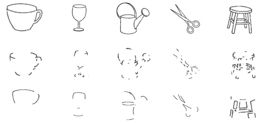
Figure 15.1 Illustration of the importance of corners to recognize objects as opposed to edges (illustration from Biederman [5]).

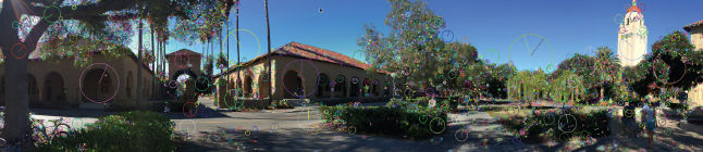
Figure 15.2 Illustration of the keypoints extracted over an image using the implementation of the SIFT [7] algorithm available in Ref. [8]. Each circle represent a keypoint. The radius of the circle corresponds to the image patch used to describe the keypoint. The radius within each circle describes the orientation of the keypoint. More details are available in Section 15.4

In this chapter, we describe methods to extract and represent keypoints. We propose to highlight the design choices that are not contradictory to our current understanding of the human visual system (HVS). We are far from claiming any biological findings, but it is worth mentioning that state-of-the-art keypoint extraction and representation can be motivated from a biological standpoint. The chapter is structured as follows: first, we briefly define some terminologies for the sake of clarity. Then, we present a quick overview of our current understanding of the HVS. We highlight models and operations within the front end of the visual system that can inspire the computer vision community to design algorithms for the detection and encoding of keypoints. In Sections 15.4 and 15.5, we present details behind the state-of-the-art algorithms to extract and represent keypoints, although it is out of the scope of this chapter to go into intricate details. We nonetheless emphasize the design choices that could mimic some operations within the human visual system. Finally, we present a new evaluation framework to get additional insight on the performance of a descriptor. We show how to reconstruct a keypoint descriptor to qualitatively analyze its behavior. We conclude by showing how to design a better image classifier using the reconstructed descriptors.

15.2 Definitions

Several terminologies have been used in various communities to describe similar concepts. For the sake of clarity, we briefly define the following terms:

Definition 1

A keypoint is a salient image point that visually stands out and is likely to remain stable under any possible image transformation such as illumination change, noise, or affine transformation to name a few.

The image patch surrounding the keypoint is described by compiling a vector given various image operators. The patch size is given by a scale space analysis that is in practice 1–10% of the image size. In the literature, a keypoint can also be referred to as an interest point, local feature, landmark, or an anchor point. The terms keypoint detector or extractor have often been used interchangeably, although the latter is probably more correct.

The equivalent biological processes of extraction and encoding of keypoints take place in the front end of the HVS, possibly as early as in the retina.

Definition 2

The front end of the visual system consists of its first few layers of neurons, from the retina photoreceptors to the primary visual cortex located in the occipital lobe of the brain.

Definition 3

The region over which a retinal ganglion cell (RGC) responds to light is called the receptive field of that cell (see Figure 15.5) [9].

The terms biologically inspired, biomimicking, or biologically plausible have similar meanings and will sometimes be used interchangeably. In this chapter, we will be drawing analogies with the behavior of the front end of the visual system in general, and the retina in particular.

15.3 What Does the Frond-End of the Visual System Tell Us?

15.3.1 The Retina

The retina is a thin layer of tissue which lines the back of the eye (see Chapters 1 and 2). It is responsible for transducing visual information into neural signals that the brain can process. A rough analogy would be that the retina is the “CCD camera” of the visual system, even though it does much more than capture a per-pixel representation of the visual world [10]. In recent years, neuroscientists have taken significant steps toward understanding the operations and calculations which take place within the human retina, that is, how images could be transmitted to the brain. The mammalian retina itself has a layered structure, in which only three types of cells, the rod and cone photoreceptors, as well as the much rarer intrinsically photosensitive RGCs, are sensitive to light [11–13]. Intrinsically, photosensitive RGCs are not thought to be involved in the image-forming pathways of the visual system, and instead are thought to play a role in synchronizing the mammalian circadian rhythm with environmental time. We therefore ignore them when describing the image encoding properties of the retina.

15.3.2 From Photoreceptors to Pixels

The photoreceptors can loosely be thought of as the “pixels” of the visual system (see Figure 15.3). They are indirectly connected to the RGCs whose axons form the optic nerve via a finely tuned network of neurons, known as the horizontal, bipolar, and amacrine cells. The bipolar cells are responsible for vertical connectionsthrough the retinal network, with horizontal and amacrine cells providing lateral connections for comparison of neighboring signals. RGCs output action potentials (colloquially referred to as “spikes”, which they “fire”) to the brain. They consist of binary, on or off signals, which the RGCs can send at up to several hundred hertz. By the time visual signals leave the retina via the optic nerve, a number of features describing the image have been extracted, with remarkably complex operations sometimes taking place: edge detection across multiple spatial scales [14], but also motion detection [15], or even segregation of object and background motion [16]. At the output of the retina, at least 17 different types of ganglion cells have extracted different spatial and temporal features of the photoreceptor activity patterns [17] over regions of the retina that have little to no overlap for a given ganglion cell type, thereby efficiently delivering information to the subsequent stages of the visual system [18]. It is worth noting that the retina does not respond to static images and instead transmits an “event-based” representation of the world to the visual cortex, where these events correspond in their simplest form to transitions from light to dark (OFF transitions), dark to light (ON transitions), or to the more complex signals mentioned in the above.

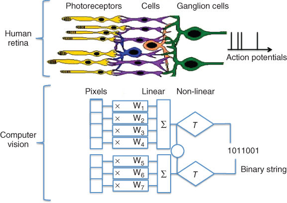
Figure 15.3 From the retina to computer vision: the biological pathways leading to action potentials can be emulated by a linear nonlinear cascade.

[Upper part of the image is a courtesy of the book Avian Visual Cognition by R. Cook]

15.3.3 Visual Compression

The visual system in general, and the retina, in particular, is an exquisitely and precisely organized system, from spatial and temporal points of view. While there are more than 100 million photoreceptors in the human eye, including approximately 5 million cone photoreceptors, the optic nerve only contains about 1 million axons, indicating that a large part of compression of the visual information takes place before it even leaves the eye. In all but the most central regions of the retina—the fovea—several photoreceptors influence each ganglion cell.

15.3.4 Retinal Sampling Pattern

Anatomically, the retina is segmented into four distinct concentric regions, defined by their distance from the central region of the retina, known as the foveola (see Figure 15.4(a)). High-resolution vision is provided by the foveola. The fovea surrounds the foveola and contains the RGCs which process the visual information captured by the cone photoreceptors located in the foveola. The foveola is indeed completely devoid of cells other than cone photoreceptors and Müller cells, which provide structural integrity to the tissue. An intermediate area, the parafoveal region, retains a relatively high RGC density and visual acuity. Both of these decrease to a minimum in the high-eccentricity perifoveal areas. In the periphery, rod photoreceptors form the majority of light-sensitive cells. Combined with a high convergence of the visual pathways, which results in high amplification of the visual signals, this makes the peripheral retina highly sensitive and efficient in low-illumination conditions, even if acuity leaves to be desired in it.

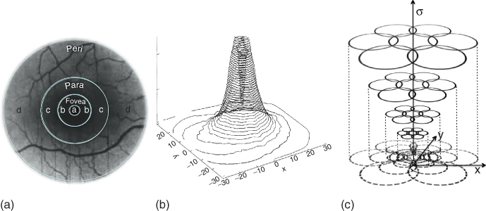
Figure 15.4 In the primate visual system, the fovea is the region of highest visual acuity. The RGCs connected to these photoreceptors are displaced in a belt which surrounds the foveola. (a) Illustration of the anatomical description of the retinal areas. The mean radial values of each of the retina areas are fovea: 1 mm; para: 3 mm; and peri: 5 mm. (b) The density of the RGC exponentially increases when moving toward the foveola [19]. The parafoveal area provides an area of intermediary visual acuity, while the low-resolution perifoveal area provides the visual system with a highly compressed, but also highly sensitive representation of the world. (c) In each region of the retina, a multiscale representation of the visual system further takes place, with different functional classes of RGCs extracting information at different spatial scales.

In the fovea, there is a one-to-one connection between individual photoreceptors and RGCs [20]. As the distance to the foveola increases, RGCs connect to more and more photoreceptors and consequently, image compression increases and visual acuity diminishes (Figure 15.4(b)). In the most peripheral regions of the retina, the midget ganglion cells, which are the smallest RGCs and thought to be responsible for the low-acuity visual pathways, can be connected to upward of 15 individual cone photoreceptors [9].

15.3.5 Scale-Space Representation

The fine-to-coarse evolution of acuity across the visual field suggests that the retina captures a multiscale representation of the world. The local spatial organization of the retina further reinforces this idea. At any point in the retina, each cone photoreceptor connects to multiple RGCs via a network of bipolar and amacrine cells. Different functional types of RGCs connect to different numbers of photoreceptors, resulting in a local multiscale representation of the visual signals [9], with so-called midget cells extracting information at finer visual scales, while so-called parasols encode a coarser description of the images (see Figures 15.4(c) and 15.5).

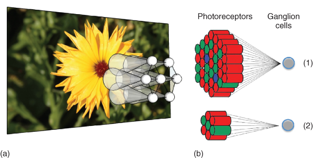
Figure 15.5 (a) Schematic representation of seven ganglion cells and their receptive fields, sampling from neighboring regions of an image (image courtesy of [21]). (b) In the perifoveal area, RGC-receptive fields are large and consist of many photoreceptors (1). As eccentricity decreases, the number of photoreceptors influencing RGCs decreases (2).

15.3.6 Difference of Gaussians as a Model for RGC-Receptive Fields

Receptive fields of RGCs consist of a central disk, the “center,” and a surrounding ring, the “surround.” The center and the surround are antagonistic, in that they respond to light increments of opposite polarity. An RGC that responds to light transitions from dark to light over its center will respond to transitions from light to dark over its surround. Such a cell is called an ON-center OFF-surround RGC, often conveniently shortened to “OFF RGC”. Conversely, OFF-center ON-surround, or ON RGCs, also exist. The center–surround shape of an RGC-receptive field is classically modeled as a difference of Gaussians (DoG) [22, 23] (see Section 15.4 for more details on the DoG). While this model fails to capture the fine structure of receptive fields [9], it appears to accurately describe the relative weighting of center and surround cells at coarser scales.

15.3.7 A Linear Nonlinear Model

While differences of Gaussians can describe retinal ganglion-cell-receptive fields relatively well on average, the retina does not behave like a simple linear system in general. A classical computational description of the retina [24] consists of a linear–nonlinear filter cascade known as the LN model (see Figure 15.6(a)), sometimes extended to take into account couplings between adjacent neurons and the non-Poisson stochastic firing patterns of the RGCs. The extended version of the LN model is known as the generalized linear model (GLM). In the LN model, a spatial filter mask extracts a region of interest over the image, and the result is transformed into a stochastic neural firing rate by the nonlinearity. This filter is typically chosen to be an exponential. In computer vision, it is possible to adopt a similar approach for extracting and representing features, as shown on Figure 15.3.

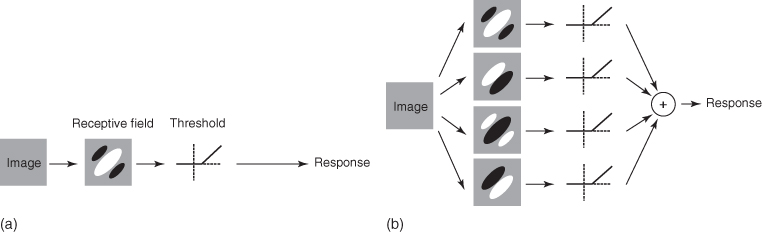
Figure 15.6 Illustration of the simple and complex cells proposed by Movhson et al. [25]. Image courtesy of [26]. (a) Simple cells are modeled using a linear filter followed by a rectifying nonlinearity. (b) For complex cells, models start with linear filtering by a number of receptive fields followed by rectification and summation.

Today, researchers are probing the retina at the single-photoreceptor level [9], measuring cells' responses to various stimuli, and trying to develop a precise understanding of how the retina extracts visual information across functional cell types.

15.3.8 Gabor-Like Filters

Further in the visual system, Hubel and Wiesel, Nobel Prize winners, discovered through seminal studies [27] that in the visual cortex of the cat, there exist cells that respond to very specific sets of stimuli. They separated neurons in the visual cortex into two different functional groups. For simple cells, responses can be predicted using a single linear filter for their receptive field, followed by a unique nonlinearity. For complex cells the response cannot be predicted using a single linear–nonlinear cascade (see Figure 15.6(b)).

Simple cells have the following properties:

· The spatial regions of the visual field over which inputs to the cell are excitatory and inhibitory are distinct.

· Spatially distinct regions of the receptive field add up linearly.

· Excitatory and inhibitarory regions balance each other out.

As a consequence, it is possible to predict the response of these cells remarkably well, using a simple linear–nonlinear model.

In 1987, Jones and Palmer performed extensive characterization of the functional receptive fields of simple cells, and found remarkable correspondence between measured receptive fields and two dimensional Gabor filters [28], thereby suggesting that the visual system adopts a sparse and redundant representation of visual signals (see Chapter 14). Building on these findings, Olshausen and Field demonstrated in 1996 that a learning algorithm that attempts to find a sparse linear code for natural scenes will lead to Gabor-like filters, similar to those found in simple cells of the visual cortex [29] (see Chapter 14). Gabor filters have since been widely adopted by the computer vision community.

15.4 Bioplausible Keypoint Extraction

The computer vision community has developed many algorithms over the past decades to identify keypoints within an image. In 1983, Burt and Adelson [30] built a Laplacian pyramid for coarse-to-fine extraction of keypoints. Since then, new methods based on multiscale Laplacian ofGaussians (LoG) [31], DoG [32], or Gabor filters [33] have been proposed. DoG is an approximation of LoG which was proposed to speed up long computation times associated with LoGs. Grossberg et al. [34] extended the DoG to directional differences-of-offset-Gaussians (DOOG) to improve the extraction step.

A popular method for keypoint extraction consists of computing the first-order statistics from zero-crossing of DoGs at different scales [35]. The scale-invariant feature transform (SIFT) [7] uses such an approach and is still one of the most used detectors after 15 years of research in the field.

15.4.1 Scale-Invariant Feature Transform

The SIFT consists of the following steps:

1. Compute the DoG of the image (see Figure 15.7).

2. Keypoints are the local maxima/minima of the DoG in scale space.

3. Use a Taylor expansion to interpolate an accurate position of the keypoint at a subpixel accuracy. It is similar to fitting a 3D curve to get location in terms of where is the pixel location and the Gaussian variance (referred to as scale). )

4. Discard keypoints along edges by discarding points with high ratio between the principal curvatures. The principal curvatures can be computed from the Hessian matrix.

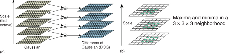
Figure 15.7 Illustration of the scale-space computation with DoG used in SIFT (a). We also illustrate the neighborhood used to compute the local maxima/minima (b). Image courtesy of [7].

Such a method leads to keypoints that are scale invariant. In general, basic keypoint extraction methods require the computation of image derivatives in both the x and y direction. The image is convolved with derivatives of Gaussians. Then, the Hessian matrix is formed, representing the second-order derivative of the image. It describes the local curvature of the image. Finally, the maxima of the determinant of the Hessian matrix are interpolated. A very popular fast implementation of such an algorithm was proposed by Bay et al., and was called speeded-up robust features (SURF) [36].

15.4.2 Speeded-Up Robust Features

The algorithm behind SURF is the following:

1. Compute the Gaussian second-order derivative of the image (instead of the DoG in SIFT).

2. A non-maximum suppression algorithm is applied in neighborhoods (position and scale).

3. The maxima of the determinant of the Hessian matrix are interpolated in space and scale.

Both SIFT and SURF find extrema at subsampled pixels that can adjust accuracy at larger scales. Agrawal et al. [37] use simplified center–surround filters (squares or octagons instead of circles) to approximate the Laplacian in an algorithm referred to as the center surround extrema (CenSurE) (see Figure 15.8).

Figure 15.8 Illustration of various type of center–surround filters used in the CenSure method [37]. (a) Circular filter. (b) Octagonal filter. (c) Hexagonal filter. (d) Box filter.

15.4.3 Center Surround Extrema

The CenSurE algorithm is as follows:

1. Octagonal center–surround filters of seven different sizes are applied to each pixel.

2. A non-maximal suppression algorithm is performed in a neighborhood.

3. Points that lie along the lines are rejected if the ratio of the principal curvature is too big. The filtering is done using the Harris method [38].

Although CenSurE was designed for speed, simpler and faster methods exist that also use circular patterns to evaluate the likelihood of having a keypoint. Rosten and Drummond [39] proposed a fast computational technique called features from accelerated segment test (FAST).

15.4.4 Features from Accelerated Segment Test

The FAST uses binary comparisons with each pixel in a circular ring around the candidate pixel. It uses a threshold to determine whether a pixel is less than the center pixel. The second derivative is not computed as it is in many state-of-the-art methods. As a result, it can be sensitive to noise and scale.

In brief, state-of-the-art keypoint extractor algorithms rely on methods for which parallels can be drawn with the way the HVS operates. These methods mainly study the gradient of the image with LoG, its approximated version with DoG, or center–surround filters. Gabor-like keypoint detectors were proposed in 1992 to compute local energy of the signal [40, 41]. In this framework, a keypoint is the maximum of the first- and second-order derivatives with respect to position. A multiscale strategy is suggested in Refs [42, 43]. Note that Gabor functions are more often used to represent the keypoints as opposed to extracting them.

15.5 Biologically Inspired Keypoint Representation

15.5.1 Motivations

In computer vision, the keypoint location itself is not informative enough to solve retrieval or recognition tasks. A vector is computed for each keypoint to provide information about the image patch surrounding the keypoint. The patch can be described densely with Gabor-like filters or sparsely with Gaussian kernels.

15.5.2 Dense Gabor-Like Descriptors

It is quite common to use the response to specific filters to describe a patch. The same filters can be applied for many different orientations. In the 1990s, Freeman and Adelson [44] used steerable filters to evaluate the response of an arbitrary orientation by interpolation from a small set of filters. As mentioned in Section 15.3, the cells' responses in the HVS can be seen as kernels. While there is no general consensus in the research community on the precise nature of the kernels, there is a convergence toward kernels that are roughly shaped like Gabor functions, derivatives, or differences of round or elongated Gaussian functions.

Over the past decades, the most common descriptors have been those modeling the gradient responses over a set of orientations. Indeed, the most popular keypoint descriptor has been the SIFT representation [7] which uses a collection of histogram of oriented gradients (HOG). Such a feature counts occurrences of gradient orientations in an image patch. In practice, the orientations are quantized into eight bins. Each bin can be seen as the response to a filter, that is, a simple cell. Figure 15.9 illustrates how a HOG can be seen as the responses of a set of simple cells.

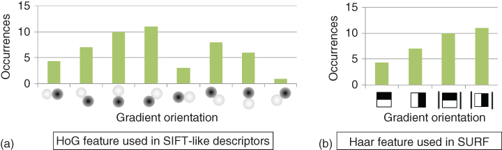
Figure 15.9 Illustration of the filter responses used to describe SIFT [7] (a) and (b) SURF [36] keypoints.

15.5.2.1 Scale-Invariant Feature Transform Descriptor

The SIFT description vector is obtained as follows:

1. Compute the gradient magnitude and direction for every pixel of the patch surrounding the keypoint. Note that a Gaussian weighting function is applied to emphasize the importance of pixels near the keypoint location.

2. The image patch is segmented into cells. The eight-bin HOG feature is computed for each cell.

3. The vector is sorted given the highest orientation and normalized to be less sensitive to illumination changes.

Different variants of the SIFT descriptor have been proposed in the literature such as PCA-SIFT [45], or GLOH [46]. The former reduces the descriptor size from 128 to 36 dimensions using principal component analysis (PCA). The latter uses a log-polar binning structure instead of the four quadrants used by SIFT (see Figure 15.10). GLOH uses spatial bins of radius 6, 11, and 15, with eight angular bins, leading to a 272-dimensional histogram. The descriptor size is further reduced from 272 to 128 using PCA.

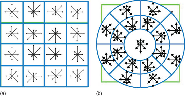
Figure 15.10 Comparison between the (a) SIFT [7] and (b) GLOH [46] strategies to segment an image patch into cells of HOG.

Although it is well accepted in the computer vision community that HOG-like descriptors are powerful features, their performance varies with respect to the number of quantization levels, sampling and overlapping strategies (e.g., polar [46] vs rectangular [7]), and whether the gradient is signed or unsigned. Bay et al. [36] propose to approximate the HOG representation with Haar-like filters to describe SURF keypoints.

15.5.2.2 Speeded-Up Robust Features Descriptor

The SURF description vector is obtained as follows:

1. A Gaussian-weighted Haar wavelet response in the x and y directions is applied every 30°to identify the orientation of the keypoint.

2. The region surrounding the keypoint is broken down into a grid. In each cell, the response in the x and y directions to Haar-wavelet features are added together. The sum of the absolute values is computed to form a element vector.

3. This vector is then normalized to be invariant to changes in contrast.

Figure 15.9 illustrates the SIFT and SURF description vectors.

15.5.3 Sparse Gaussian Kernels

In the signal processing community, researchers have recently started trying to reconstruct signals given a sparsity constraint with respect to a suitable basis. Interestingly, many signals and phenomena can be represented sparsely, with only a few nonzero (or active) elements in the signal. Images are in fact sparse in the gradient domain. They are considered as piecewise smoothed signals. As a result, we do not need to compute the responses of filters over all locations.

Calonder et al. [47] showed that computing the Gaussian difference between a few random points within the image patch of a keypoint is good enough to describe it for keypoint matching purposes. In addition, the Gaussians do not need to be concentric. They further use the sign of the difference to represent the keypoint, leading to a very compact binary descriptor. This method belongs to the family of descriptors coined local binary descriptors (LBDs).

15.5.3.1 Local Binary Descriptors

Local Binary Descriptors perform the following steps times:

1. Compute the Gaussian average at two locations and within the image patch with variance and , respectively.

2. Compute the difference between these two measurements

3. Binarize the resulting difference by retaining the sign only.

There are several considerations in the design of LBD. How should we select the Gaussians (locations and variances)? How many times should we perform the steps (i.e., what is a good size for )? What is the optimal sampling of the image patch to encode as much information as possible with the lowest number of comparison (i.e., bits)?

Interestingly, LBD can be compared to the linear nonlinear filter cascades present in the HVS (see Figure 15.3). Alahi et al. [48] propose an LBD inspired by the retinal sampling grid. There are many possible sampling grids to compare pairs of Gaussian responses: for instance, BRIEF [47] and ORB [49] use random Gaussian locations with the same fixed variance. BRISK [50] uses a circular pattern with various Gaussian sizes. Alahi et al. proposed the fast retina keypoint (FREAK) [48] which uses a retinal sampling grid, as illustrated in Figure 15.11. They heuristically show that the matching performance increases when a retinal sampling grid is used as compared to previous strategies (see Figure 15.12).

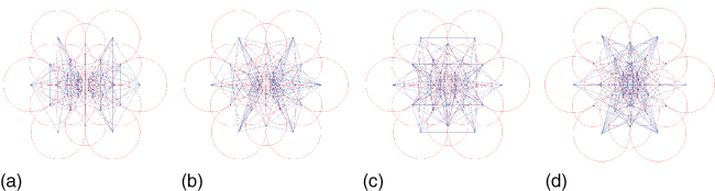
Figure 15.11 Illustration of the retinal sampling grid used in FREAK [48]. Each line represents the pairs of Gaussians selected to measure the sign of their difference. The first cluster mainly involves perifoveal receptive fields and the last ones foveal ones.

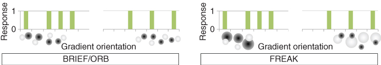
Figure 15.12 Illustration of the filter responses used to describe the binaries' descriptors (BRIEF [47], ORB [49], and FREAK [48]).

15.5.3.2 Fast Retina Keypoint Descriptor

The FREAK uses a retinal pattern to promote a coarse-to-fine representation of a keypoint. Figure 15.11 illustrates the topology of the Gaussians kernels. Each circle represents the 1-standard deviation contour of a Gaussian applied to the corresponding sampling points. The pattern is made of one central point and seven concentric circles of six points each, with circles being shifted by 30°with respect to the contiguous ones. The FREAK pattern can be seen as a multiscale description of the keypoint image patch. The coarse-to-fine representation allows the keypoint to be matched in a cascade manner, that is, segment after segment, to speed up the retrieval step. Given the retinal pattern, thousands of pairs of Gaussian responses can be measured. Alahi et al. [48] use a learning step similar to ORB [49] to select a restricted number of pairs. The selection algorithm is as follows:

1. Form a matrix representing several hundred thousands of keypoints. Each row corresponds to a keypoint represented with its large descriptor made of all possible pairs in the retina sampling pattern illustrated in Figure 15.11. There are more than 900 possible pairs with 4 dozens of Gaussians.

2. Compute the mean of each column. In order to have a discriminant feature, high variance is desired. A mean of 0.5 leads to the highest variance of a binary distribution.

3. Order the columns with respect to the highest variance.

4. Keep the best column (mean of 0.5) and iteratively add the remaining columns having low correlation with the selected columns.

Figure 15.11 illustrates the pairs selected by grouping them into four clusters (128 pairs per group)¹. Note that using more than 512 pairs did not improve the performance of the descriptor. The first cluster involves more of the peripheral Gaussians and the last one, the central ones. The remaining clusters highlight activities in the remaining area of the retina (i.e., the parafoveal are). The obtained clusters seem to match the behavior of the human eye. We first use the perifoveal receptive fields to estimate the location of an object of interest. Then, validation is performed with the more densely distributed receptive fields inthe foveal area. Although the used feature selection algorithm is greedy, it seems to match our understanding of the model of the human retina. Furthermore, it is possible to take advantage of the coarse-to-fine structure of the FREAK descriptor to match keypoints.

15.5.3.3 Fast Retina Keypoint Saccadic Matching

To match FREAK keypoints, Alahi et al. [48] have proposed to mimic saccadic search by parsing the descriptor in several steps. They start by matching with the first 128 bits of the FREAK descriptor representing coarse information. If the distance is smaller than a threshold, they further continue the comparison with the rest of the binary string to analyze finer information. As a result, a cascade of comparisons is performed decreasing the time required for the matching step with respect to other LBD. More than 90% of the candidates are discarded with the first 128 bits of the FREAK descriptor using a threshold large enough to speed up matching but not to alter the final result. Figure 15.13 illustrates the saccadic match. For visualization purposes, an object of interest is represented with a single FREAK descriptor of the size of its bounding circle (Figure 15.13(a)). Then, a new image is searched for the same object. All candidate image regions (a regular grid of keypoints at three different scales) are also described with a single descriptor of the size of the candidate region. The first cascade (Figure 15.13(b) and (d)) (first 16 bytes) discards many candidates and selects very few of them to compare with the remaining bytes. In Figure 15.13(e), the last cascade (Figure 15.13c) has correctly selected the locations of our object of interest despite the changes of illuminations and viewpoints.

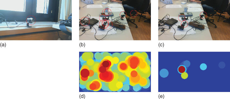
Figure 15.13 Illustration of the FREAK cascade matching. (a) An object of interest. (b) Ten best matches after the first cascade. (c) Three best matches after the last cascade. (d) Heatmap after the first cascade. (e) Heatmap after the last cascade. In (b) and (d), the distance of all regions to the object of interest is illustrated in color jet. In (c), we can see that the object of interest is located in the few estimated regions. These regions can simulate the saccadic search of the human eyes.

15.5.4 Fast Retina Keypoint versus Other Local Binary Descriptors

All LBDs use Gaussian responses in order to be less sensitive to noise. BRIEF [47] and ORB [49] use the same kernel for all points in the patch. To match the retina model, FREAK uses different kernels for every sample point, similar to BRISK [50]. The difference from BRISK is the exponential change in size and the overlapping kernels. It has been observed that overlapping between points of different concentric circles improves performance. One possible reason is that with the presented overlap, more information is captured. An intuitive explanation could be formulated as follows.

Let us consider the intensities measured at the receptive fields A, B, and C where

, , and .

If the fields do not overlap, then the last test is does not add any discriminant information. However, if the fields overlap partially, new information can be encoded. In general, adding redundancy allows us to use fewer receptive fields. This has been a strategy employed in compressed sensing (CS) or dictionary learning for many years. According to Olshausen and Field [51], such redundancies also exist in the receptive fields of the visual cortex.

15.6 Qualitative Analysis: Visualizing Keypoint Information

15.6.1 Motivations

In the previous sections, we presented several methods to extract and represent keypoints. It is beyond the scope of this chapter to present all possible techniques. Tuytelaars and Mikolajczyk [46] extensively describe the existing keypoint extractor techniques and their desired properties for computer vision applications such as repeatability, locality, quantity, accuracy, efficiency, invariance, and robustness. For instance, the repeatability score is computed as follows:

15.1

where refers to the number of correspondences; and are the numberof detected keypoints from an image and its transformed image , respectively. It measures whether a keypoint remains stable over any possible image transformation.

The performance of keypoint descriptors is solely compared on the basis of their performance in full grown, end-to-end machine vision tasks such as image registration or object recognition, as in Ref. [49]. While this approach is essential for developing working computer vision applications, it provides little hindsight on the type and quantity of local image content that is embedded in the keypoint under test.

We dedicate the last section of this chapter to the presentation of two lines of work that bring a different viewpoint on local image descriptors. In the first part, we see a method to invert binarized descriptors, thus allowing a qualitative analysis of the differences between BRIEF and FREAK. The second part presents an experiment that combines descriptor inversion, crowd intelligence, and some psychovisual representations to build better image classifiers.

Eventually, these research projects will yield a better methodology for developing image part descriptors that are not only accurate but also mimic the generalization properties experienced every day in the human mind.

15.6.2 Binary Feature Reconstruction: From Bits to Image Patches

In the preceding sections of the chapter, we learned that BRIEF and FREAK are LBDs: they produce a bitstream that should unambiguously describe local image content in the vicinity of a given keypoint. They differ only in the patch sampling strategy. While BRIEF uses fixed width Gaussians randomly spread over the patch, FREAK, on the other hand, relies on the retinal pattern and its Gaussian measurements are concentric and wider away from the patch center.

15.6.2.1 Feature Inversion as an Inverse Problem

While a detailed description of the solver used to invert binary descriptors is beyond the scope of the current chapter, we describe in this paragraph the mathematical modeling process that led to its development so that the reader can apply it to their own reconstruction problems.

Let us consider that we are given an image patch of size . We want to describe it using an LBD (be it BRIEF or FREAK) of length bits. Empirically, we obtain a component of the feature descriptor by

1. picking a location within the patch;

2. overlapping this area with a Gaussian (green area in Figure 15.14);

3. multiplying point-to-point, the value of the Gaussian with the pixel values in the patch;

4. taking the mean of these premultiplied values;

5. repeating this process with another location and another Gaussian (red area in Figure 15.14);

6. computing the difference between the green mean and the red mean;

7. assigning for the current feature vector component if the difference is positive and , otherwise.

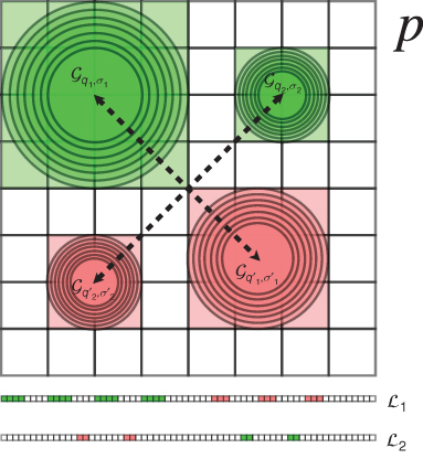
Figure 15.14 Example of a local descriptor for an pixels patch and the corresponding sensing matrix. Only two measurements of the descriptor are depicted; each one is produced by subtracting the Gaussian mean in the lower (red) area from the corresponding upper (green) one. All the integrals are normalized by their area to have values in . Below this are the corresponding vectors.

If we reshape the image patch into a column of size , steps 1–4 are mathematically represented by the dot product between a normalized Gaussian of width centered in and the patch vector . Computing steps 1–5 for different pairs of points inside a patch and taking the difference depicted in step 6 is fully represented by the linear operator defined by

15.2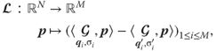

Since is linear, it can be represented as a matrix (Figure 15.14 bottom) applied to the input vectorized patch and obtained by stacking rows :

15.3

The final binary descriptor is obtained by the composition of this sensing matrix with a componentwise quantization operator defined by , so that, given a patch , the corresponding LBD reads as

Even without the binarization step, the reconstruction problem for any LBD operator is ill-posed because there are typically many fewer measurements than there are pixels in the patch. In Reference [52] pixel image patches are described using measurements only. Classically, this problem can be made tractable by using a regularized inverse problem approach: adding regularization constraints allows the incorporation of a priori knowledge about the desired solution that will compensate for the lost information. The reconstructed patches will be obtained by solving a problem made of two constraints:

· a data term that will tie the reconstruction to the input binary descriptor;

· a regularization term that will enforce some prior knowledge about the desirable properties of the reconstruction.

In order to avoid any bias introduced by a specific training set, a natural candidate for the regularization constraint is the sparsity of the reconstructed patches in some wavelet frame . This requires that the patches have only a few nonzero coefficients after analysis in this wavelet frame. A simple way to enforce this constraint is to add a penalty term that grows with the number of nonzero coefficients. Mathematically, counting coefficients can be performed by measuring the cardinality (written ) of the set they belong to. For the case at hand, let us decompose these different steps:

1. A candidate patch in a wavelet frame that is obtained by computing the matrix-vector product is analyzed.

2. The set of interest is made of the components of the vector that are nonzero.

3. We count how many of these are there: .

Variational frameworks are designed to minimize the norm of error vectors instead of the cardinality of a set. This is why these frameworks use instead the -norm of a vector, which is defined in terms of the number of its nonzero coefficients:

15.4

This assumption may seem abstract, but it amounts to say that all the spatial frequencies are not present in an image and that most of the information is carried by only a subset of them. We experience this every day, as it is one of the principles behind compression schemes such as JPEG.

As a last step, defining a normalization constraint is required. From Eq. (15.3), it is clear that an LBD is a differential operator by nature. Thus, the original values of the pixels are definitely lost and we can reconstruct their variations only. This ambiguity can be solved by arbitrarily fixing the dynamic range of the pixels to the interval and constraining the reconstructed patches to belong to the set of the patches of mean 0.5.

Finally, the reconstruction problem can be written as

15.5

The data term first applies the linear operator to the current reconstruction estimate , binarizes the result and counts how many bits are different between and the input descriptor . Eq. (15.4) is a special instance of a Lasso-type program [53] that can be solved with an iterative procedure (see Refs. [54, 55], and Chapter 14, Section 1).

15.6.2.2 Interest of the Retinal Descriptor

This has taken us a long way from keypoints and biology. We come back to our matter by picking a solver for Eq. (15.4) (see Ref. [54]). Does the resolution of the problem (15.5) exhibit meaningful differences when applied to regular keypoints or to bioinspired ones? Let us proceed to some experiments using BRIEF (for the regular one) and FREAK (for the bioinspired one).

We start by decomposing a well known image into nonoverlapping patches. Computing BRIEF and FREAK descriptors then reconstructing each patch yields the results shown in Figure 15.15. These results are strikingly different. BRIEF allows to immediately recognize the original image of Lena. The edges, however, are larger and more blurred: each reconstructed patch behaves like a large, blurred sketch of the original image content. Using FREAK instead, the reconstructed image looks like a weird patchwork. Carefully observing what happens in the center, however, shows that the original image directions are accurately reconstructed.

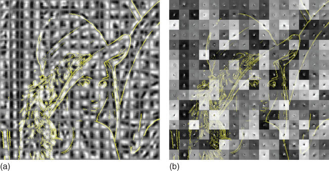
Figure 15.15 Reconstruction of Lena from binary LBDs. There is no overlap between the patches used in the experiment, thus the blockwise aspect. Yellow lines are used to depict some of the edges of the original image. In both cases, the orientation selected for the output patch is consistent with the original gradient direction. (a) BRIEF allows to recover large blurred edges, while (b) FREAK concentrates most of the information in the center of the patch.

When considering the retinal pattern from Figure 15.11, this effect is quite intuitive. In this sampling, the outer cells have a coarser resolution than the innermost ones. Thus, the image geometry encoded in a FREAK descriptor has a very coarse scale near the orders of the patch and becomes more and more sensitive when moving to the center. Owing to the random nature of the measurement positions inside a patch, BRIEF does consider all the content equally and is not biased toward its center.

Because FREAK focalizes its attention to an area near the center of the patch, it encodes finer details in the descriptor than BRIEF. This is confirmed by the experiment shown in Figure 15.16. In this second experiment, the patches to reconstruct are first selected by the FAST keypoint detector. Since FAST points tend to aggregate near corners and edges, there is a large overlap between the patches that discards the block artifacts from Figure 15.15. The capability of FREAK to encode fine edge information is well illustrated by this example. The fine pattern of the tissue can be correctly perceived while it is blurred out by BRIEF. Even the more variable orientations of the hat feathers of Lena can be reconstructed.

Figure 15.16 Reconstruction of LBDs centered on FAST keypoints only. Columns: Lena image, its zoom version; Barbara image, and its zoom version. (a) using BRIEF. (b) using FREAK. Since the detected points are usually very clustered, there is a dense overlap between patches, yielding a reconstruction that is visually better than the one in Figure 15.15.

15.6.3 From Feature Visualization to Crowd-Sourced Object Recognition

A key difference between the human mind and machine vision classifiers is the ability of humans to easily generalize their knowledge to never-seen instances of objects. A kind of brute force approach to tackle this problem is, of course, to make training sets bigger, but this approach will be inherently limited by practical cost issues and by more subtle effects of low occurrence rates for some objects of interest. In Reference [56], Vondrick et al. propose an original way around this problem that associates the results of a feature inversion algorithm and human psychophysics tools to train and build better classifiers that are capable of recognizing objects without ever seeing them during the training phase.

How did they manage to do so? Their work is based on the following observation: if we generate hundreds or thousands of noise images of a given size, then some of them will contain accidental shapes that look like actual objects or geometric figures that can be detected by human observers. This principle is used, for example, in studies of the HVS [57].

Of course, generating random images and waiting for humans to see anything inside would also be time- and money-consuming, and this would still require features to be computed and selected from these random images. Furthermore, these random noise images might not be very efficient, as they would probably lack geometric features such as edges when generated as pixelwise random noise. However, given a feature inversion algorithm, it is possible to reconstruct image parts from random feature vectors and submit these images to human viewers instead.

Thus, Vondrick et al. selected the popular HOG [58] and CNN [59] object descriptors that are used in most state-of-the-art object visual classifiers. They then took the following steps:

1. Random realizations of HOG and CNN [59] feature descriptors were generated.

2. A feature inversion algorithm was fed with these random vectors. The feature inversion method that they used is described in Ref. [60].

3. These reconstruction results were submitted to human viewers on a large-scale sample using Amazon Mechanical Turk.² These workers were tasked with identifying the category (if any) of the object inside each picture.

Finally, they trained a visual object classifier that approximates the average human worker decision between object categories and pure noise. This is an imaginary classifier, as it has never seen a real object in its training phase but only hallucinated objects instead.

The reference images used by the imaginary classifiers for different object classes can be seen in Figure 15.17. It is interesting to note that the usual geometric shape of the object is retrieved in each case: cars and televisions have corners and are roughly rectangular, while bottles, persons, or fire hydrants are vertically elongated. Since CNN also encode the original color of the images, it is remarkable that the fire hydrant model selected from the human workers turned out to be red, as one might expect.

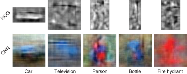
Figure 15.17 Decision boundaries acquired from Mechanical Turk workers after presenting them inverted random image descriptors. Illustration reprinted from Vondrick et al. [56].

Table 15.1 shows the average precision of these object classifiers on the PASCAL VOC 2011 challenge compared to the output of a purely random classifier. In most cases, the imaginary classifier significantly outperforms the random classifier, showing that relevant information was transferred from the human viewers to the automatic system. Vondrick et al. also managed to train classifiers as a compromise between an actual training set and hallucinated images. When the size of the training set grows, the benefits of the imaginary classifiers vanish. This is, however, a promising first step to building better object recognition systems from a smaller number of examples and future research may succeed in transferring the generalization skills of the human mind to automatic systems.

Table 15.1 Average precision of imaginary classifiers (trained without any real object images) on the PASCAL VOC 2011 dataset. Boldface numbers emphasize cases where the imaginary classifier clearly outperforms a random classifier. Reprinted from Vondrick et al. [56]

As a closing remark, recall that CNN were designed to mimic the human visual cortex [59]. Using the training method proposed by Vondrick et al., we can then build an image recognition system whose behavior reproduces that of the human brain and which exploits information from a human crowd although it has never seen a real image.

15.7 Conclusions

Keypoint extraction and representation techniques are usually the first step toward more challenging computer vision tasks such as object retrieval or 3D reconstruction. Such a low-level feature extraction step becomes more practical if its computational cost is low. Such a condition has led to the recent designs of fast algorithms for computing binary descriptors that are consistent with our current understanding of the front end of the visual system. However, we would like to point out to the reader that many other informative statistical approaches exist to describe an image patch, fusing several low-level features such as the covariance descriptor [61] or image moments [62], to name a few. These methods are typically computationally more costly than the binary descriptors. In the last section of this chapter, we saw that such binary features can be inverted to yield plausible visual reconstructions. This process can be used not only to better understand differences between descriptors but also to open up novel and promising approaches to developing complete machine vision systems.

We would like to conclude this chapter by sharing some links on available codes to run the presented methods in this chapter. First, codes are available in matlab [63] or C/C++/python [8] to extract and represent keypoints with the presented algorithms. Second, the source code to generate the experiments of the feature inversion algorithms are available online as well [64] and [65]. The detailed mechanics of both techniques are presented in Refs [54, 66] for LBD and Ref. [60] for HOG/CNN. The LBD reconstruction framework makes heavy use of results and tools from an emerging field called compressive sensing(CS), and in particular 1-bit CS. The Rice University maintains a comprehensive list of CS resources at the address [67], including 1-bit CS references. Finally, deriving actual computer vision algorithms from psychovisual studies is an arduous task although the whole field of research is impregnated with David Marr's primal sketch. Readers interested in an alternative way of linking psychological theories of perception and mathematical algorithms can find some alternative inspiration in A. Desolneux's work regrouped in Ref. [68]. This work tries to estimate salient structures from noise, but also relies on the Gestalt theory (as formalized by Wertheimer and Kanizsa) to model the human perception. This allows the authors to derive robust, parameter-less algorithms to detect low-level features inimages.

References

1. 1. Jepson, L.H., Hottowy, P., Mathieson, K., Gunning, D.E., Dabrowski, W., Litke, A.M., and Chichilnisky, E.J. (2013) Focal electrical stimulation of major ganglion cell types in the primate retina for the design of visual prostheses. J. Neurosci., 33 (17), 194–205.

2. 2. Krizhevsky, A., Sutskever, I., and Hinton, G.E. (2012) Imagenet classification with deep convolutional neural networks. Advances in Neural Information Processing Systems, pp. 1097–1105.

3. 3. Russakovsky, O., Deng, J., Su, H., Krause, J., Satheesh, S., Ma, S., Huang, Z., Karpathy, A., Khosla, A., Bernstein, M., Berg, A.C., and Fei-Fei, L. (2015) ImageNet Large Scale Visual Recognition Challenge. International Journal of Computer Vision (IJCV), 1–42, doi: 10.1007/s11263-015-0816-y.

4. 4. Neisser, U. (1964) Visual Search, Scientific American.

5. 5. Biederman, I. (1987) Recognition-by-components: a theory of human image understanding. Psychol. Rev., 94 (2), 115.

6. 6. Shi, J. and Tomasi, C. (1994) Good features to track. 1994 IEEE Computer Society Conference on Computer Vision and Pattern Recognition, 1994. Proceedings CVPR'94, IEEE, pp. 593–600.

7. 7. Lowe, D.G. (1999) Object recognition from local scale-invariant features. The Proceedings of the 7th IEEE International Conference on Computer vision, 1999, vol. 2, IEEE, pp. 1150–1157.

8. 8. Opencv's Features2d Framework, http://docs.opencv.org/ (accessed 30 April 2015).

9. 9. Field, G.D., Gauthier, J.L., Sher, A., Greschner, M., Machado, T.A., Jepson, L.H., Shlens, J., Gunning, D.E., Mathieson, K., Dabrowski, W. et al. (2010) Functional connectivity in the retina at the resolution of photoreceptors. Nature, 467, 673–677.

10.10. Gollisch, T. and Meister, M. (2010) Eye smarter than scientists believed: neural computations in circuits of the retina. Neuron, 65 (2), 150–164.

11.11. Granit, R. (1947) Sensory Mechanisms of the Retina, Oxford University Press, London.

12.12. Stryer, L. (1988) Molecular basis of visual excitation, Cold Spring Harbor Symposia on Quantitative Biology, vol. 53, Cold Spring Harbor Laboratory Press, pp. 283–294.

13.13. Berson, D.M., Dunn, F.A., and Takao, M. (2002) Phototransduction by retinal ganglion cells that set the circadian clock. Science, 295 (5557), 1070–1073.

14.14. Barlow, H.B., Fitzhugh, R., and Kuffler, S.W. (1957) Change of organization in the receptive fields of the cat's retina during dark adaptation. J. Physiol., 137, 338–354.

15.15. Borst, A. and Euler, T. (2011) Seeing things in motion: models, circuits, and mechanisms. Neuron, 71, 974–994.

16.16. Ölveczky, B., Baccus, S., and Meister, M. (2003) Segregation of object and background motion in the retina. Nature, 423, 401–408.

17.17. Field, G.D. and Chichilnisky, E.J. (2007) Information processing in the primate retina: circuit and coding. Annu. Rev. Neurosci., 30, 1–30.

18.18. Doi, E., Gauthier, J.L., Field, G.D., Shlens, J., Sher, A., Greschner, M., Machado, T.A., Jepson, L.H., Mathieson, K., Gunning, D.E., Litke, A.M., Paninski, L., Chichilnisky, E.J., and Simoncelli, E.P. (2012) Efficient coding of spatial information in the primate retina. J. Neurosci., 32 (46), 16256–16264.

19.19. Garway-Heath, D.F., Caprioli, J., Fitzke, F.W., and Hitchings, R.A. (2000) Scaling the hill of vision: the physiological relationship between light sensitivity and ganglion cell numbers. Invest. Ophthalmol. Visual Sci., 41 (7), 1774–1782.

20.20. Kolb, H. and Marshak, D. (2003) The midget pathways of the primate retina. Doc. Ophthalmol., 106 (1), 67–81.

21.21. Ebner, M. and Hameroff, S. (2011) Lateral information processing by spiking neurons: a theoretical model of the neural correlate of consciousness. Comput. Intell. Neurosci., 2011, 247879.

22.22. Dacey, D., Packer, O.S., Diller, L., Brainard, D., Peterson, B., and Lee, B. (2000) Center surround receptive field structure of cone bipolar cells in primate retina. Vision Res., 40, 1801–1811.

23.23. Enroth-Cugell, C. and Robson, J.G. (1966) The contrast sensitivity of retinal ganglion cells of the cat. J. Physiol., 187, 517–552.

24.24. Pillow, J.W., Shlens, J., Paninski, L., Sher, A., Litke, A.M., Chichilnisky, E.J., and Simoncelli, E.P. (2008) Spatio-temporal correlations and visual signalling in a complete neuronal population. Nature, 454, 995–999.

25.25. Movshon, J.A., Thompson, I., and Tolhurst, D. (1978) Spatial and temporal contrast sensitivity of neurones in areas 17 and 18 of the cat's visual cortex. J. Physiol., 283 (1), 101–120.

26.26. Carandini, M. (2006) What simple and complex cells compute. J. Physiol., 577 (2), 463–466.

27.27. Hubel, D.H. and Wiesel, T.N. (1962) Receptive fields, binocular interaction and functional architecture in the cat's visual cortex. J. Physiol., 160 (1), 106.

28.28. Jones, J.P. and Palmer, L.A. (1987) An evaluation of the two-dimensional Gabor filter model of simple receptive fields in the cat striate cortex. J. Neurophysiol., 58 (6), 1233–1258.

29.29. Olshausen, B.A. and Field, D.J. (1996) Emergence of simple-cell receptive field properties by learning a sparse code for natural images. Nature, 381, 607–609.

30.30. Burt, P.J. and Adelson, E.H. (1983) The Laplacian pyramid as a compact image code. IEEE Trans. Commun., 31 (4), 532–540.

31.31. Sandon, P.A. (1990) Simulating visual attention. J. Cognit. Neurosci., 2 (3), 213–231.

32.32. Gaussier, P. and Cocquerez, J.P. (1992) Neural networks for complex scene recognition: simulation of a visual system with several cortical areas. International Joint Conference on Neural Networks, 1992. IJCNN, vol. 3, IEEE, pp. 233–259.

33.33. Azzopardi, G. and Petkov, N. (2013) Trainable COSFIRE filters for keypoint detection and pattern recognition. IEEE Trans. Pattern Anal. Mach. Intell., 35 (2), 490–503.

34.34. Grossberg, S., Mingolla, E., and Todorovic, D. (1989) A neural network architecture for preattentive vision. IEEE Trans. Biomed. Eng., 36 (1), 65–84.

35.35. Brecher, V.H., Bonner, R., and Read, C. (1991) Model of human preattentive visual detection of edge orientation anomalies. Orlando'91, Orlando, FL, International Society for Optics and Photonics, pp. 39–51.

36.36. Bay, H., Tuytelaars, T., and Van Gool, L. (2006) SURF: speeded up robust features, Computer Vision–ECCV 2006, Springer-Verlag, pp. 404–417.

37.37. Agrawal, M., Konolige, K., and Blas, M.R. (2008) CenSurE: center surround extremas for realtime feature detection and matching, Computer Vision–ECCV 2008, Springer-Verlag, pp. 102–115.

38.38. Harris, C. and Stephens, M. (1988) A combined corner and edge detector. Alvey Vision Conference, vol. 15, Manchester, UK, p. 50.

39.39. Rosten, E. and Drummond, T. (2006) Machine learning for high-speed corner detection, Computer Vision–ECCV 2006, Springer-Verlag, pp. 430–443.

40.40. Heitger, F., Rosenthaler, L., Von Der Heydt, R., Peterhans, E., and Kübler, O. (1992) Simulation of neural contour mechanisms: from simple to end-stopped cells. Vision Res., 32 (5), 963–981.

41.41. Rosenthaler, L., Heitger, F., Kübler, O., and von der Heydt, R. (1992) Detection of general edges and keypoints, Computer Vision ECCV'92, Springer-Verlag, pp. 78–86.

42.42. Robbins, B. and Owens, R. (1997) 2D feature detection via local energy. Image Vision Comput., 15 (5), 353–368.

43.43. Manjunath, B., Shekhar, C., and Chellappa, R. (1996) A new approach to image feature detection with applications. Pattern Recognit., 29 (4), 627–640.

44.44. Freeman, W.T. and Adelson, E.H. (1991) The design and use of steerable filters. IEEE Trans. Pattern Anal. Mach. Intell., 13 (9), 891–906.

45.45. Ke, Y. and Sukthankar, R. (2004) PCA-SIFT: a more distinctive representation for local image descriptors. Proceedings of the 2004 IEEE Computer Society Conference on Computer Vision and Pattern Recognition, 2004. CVPR 2004, vol. 2, IEEE, pp. II–506.

46.46. Tuytelaars, T. and Mikolajczyk, K. (2008) Local invariant feature detectors: a survey. Found. Trends® in Comput. Graph. and Vision, 3 (3), 177–280.

47.47. Calonder, M., Lepetit, V., Strecha, C., and Fua, P. (2010) BRIEF: binary robust independent elementary features, Computer Vision–ECCV 2010, Springer-Verlag, pp. 778–792.

48.48. Alahi, A., Ortiz, R., and Vandergheynst, P. (2012) FREAK: fast retina keypoint, 2012 IEEE Conference on Computer Vision and Pattern Recognition (CVPR), IEEE, pp. 510–517.

49.49. Rublee, E., Rabaud, V., Konolige, K., and Bradski, G. (2011) ORB: an efficient alternative to SIFT or SURF. 2011 IEEE International Conference on Computer Vision (ICCV), IEEE, pp. 2564–2571.

50.50. Leutenegger, S., Chli, M., and Siegwart, R.Y. (2011) BRISK: binary robust invariant scalable keypoints. 2011 IEEE International Conference on Computer Vision (ICCV), IEEE, pp. 2548–2555.

51.51. Olshausen, B.A. and Field, D.J. (2004) What is the other 85% of V1 doing?. Prob. Syst. Neurosci., 4 (5), 182–211.

52.52. Leutenegger, S., Chli, M., and Siegwart, Y. (2011) BRISK: binary robust invariant scalable keypoints. 2011 IEEE International Conference on Computer Vision (ICCV), pp. 2548–2555.

53.53. Tibshirani, R. (1994) Regression shrinkage and selection via the lasso. J. R. Stat. Soc. Ser. B, 58, 267–288.

54.54. d'Angelo, E., Jacques, L., Alahi, A., and Vandergheynst, P. (2014) From bits to images: inversion of local binary descriptors. IEEE Trans. Pattern Anal. Mach. Intell., 36 (5), 874–887, doi: 10.1109/TPAMI.2013.228.

55.55. Jacques, L., Laska, J.N., Boufounos, P.T., and Baraniuk, R.G. (2011) Robust 1-bit compressive sensing via binary stable embeddings of sparse vectors. IEEE Trans. Inf. Theory, 59 (4), 2082–2102.

56.56. Vondrick, C., Pirsiavash, H., Oliva, A., and Torralba, A. (2014) Acquiring Visual Classifiers from Human Imagination, http://web.mit.edu/vondrick/imagination/ (accessed 30 April 2015).

57.57. Beard, B.L. and Ahumada, A.J. Jr. (1998) Technique to extract relevant image features for visual tasks. SPIE Proceedings, vol. 3299, pp. 79–85, doi: 10.1117/12.320099.

58.58. Dalal, N. and Triggs, B. (2005) Histograms of oriented gradients for human detection. IEEE Computer Society Conference on Computer Vision and Pattern Recognition, 2005. CVPR 2005, vol. 1, pp. 886–893, doi: 10.1109/CVPR.2005.177.

59.59. LeCun, Y., Bottou, L., Bengio, Y., and Haffner, P. (1998) Gradient-based learning applied to document recognition. Proc. IEEE, 86 (11), 2278–2324, doi: 10.1109/5.726791.

60.60. Vondrick, C., Khosla, A., Malisiewicz, T., and Torralba, A. (2013) HOGgles: visualizing object detection features. 2013 IEEE International Conference on Computer Vision (ICCV), pp. 1–8, doi: 10.1109/ICCV.2013.8.

61.61. Tuzel, O., Porikli, F., and Meer, P. (2006) Region covariance: a fast descriptor for detection and classification. Computer Vision–ECCV 2006, Springer-Verlag, pp. 589–600.

62.62. Hwang, S.K., Billinghurst, M., and Kim, W.Y. (2008) Local descriptor by Zernike moments for real-time keypoint matching. Congress on Image and Signal Processing, 2008. CISP'08, vol. 2, IEEE, pp. 781–785.

63.63. MathWorks Matlab r2014b Computer Vision Toolbox, http://www.mathworks.com/products/computer-vision/ (accessed 30 April 2015).

64.64. GitHub LBD Reconstruction Code, https://github.com/sansuiso/LBDReconstruction (accessed 30 April 2015).

65.65. Source Code to Invert Hog, https://github.com/CSAILVision/ihog (accessed 30 April 2015).

66.66. d'Angelo, E., Alahi, A., and Vandergheynst, P. (2012) Beyond bits: reconstructing images from local binary descriptors. 2012 21st International Conference on Pattern Recognition (ICPR), pp. 935–938.

67.67. Rice Compressive Sensing Resource, http://dsp.rice.edu/cs.

68.68. Desolneux, A., Moisan, L., and Morel, J.M. (2008) From Gestalt Theory to Image Analysis, Springer-Verlag.

¹ Groups of 128 pairs are considered here because of hardware requirements. The Hamming distance used in the matching process is computed by segments of 128 bits thanks to the SSE instruction set.² Amazon Mechanical Turk is a crowd-sourcing Internet marketplace that enables researchers to coordinate the use of human intelligence to perform large-scale tasks at a reduced labor cost.