Biologically Inspired Computer Vision (2015)

Part II
Sensing

Chapter 8
Plenoptic Cameras

Fernando Pérez Nava, Alejandro Pérez Nava, Manuel Rodríguez Valido and Eduardo Magdaleno Castellò

8.1 Introduction

The perceptual system provides to biological and artificial agents information about the environment in which they inhabit. This information is obtained by capturing one or more of the types of energy that surrounds them. By far, the most informative is light, electromagnetic radiation in the visible spectrum. The sun fills the earth with photons that are reflected and absorbed by the environment and finally perceived by visual sensors. This initiates several complex information processing tasks that supply the agents with an understanding of their environment. There is an enormous interest to comprehend and replicate the biological visual perceptual system in artificial agents. The first step of this process is deciding how to capture light. To design visual sensors in artificial agents, we are not constrained by evolutionary or biological reasons and we may question if it is appropriate to replicate the human visual system. Although at first sight it seems reasonable that sensors resembling our eyes are more appropriate for the tasks that we are interested for computers to automate, other eye designs present in animals or not explored by the evolution may provide better performance for some tasks.

Eye design in animals began with simple photosensitive cells to capture light intensity. From these remote beginnings, eye evolution has been guided toward increasing the information that can be extracted from the environment [1]. When photosensitive cells were placed on a curved surface, directional selectivity was incorporated to the recorded light intensity. The curvature of this inward depression increased and finally formed a chamber, with an inlet similar to a pinhole camera. Pinhole cameras face a trade-off between low light sensitivity (increasing with bigger holes) and resolution (increasing with smaller holes). The solution both in photography and animal eye evolution is the development of a lens. The resulting eye is the design found in vertebrates. The main advantages of single-aperture eyes are high sensitivity and resolution, while its drawbacks are the small size of the field of view and its large volume and weight [2]. For small invertebrates, eyes are very expensive in weight and brain processing needs, so the compound eye was developed as a different solution toward achieving more information. Rather than curving the photoreceptive surface inward, evolution has led to a surface curved outward in these creatures. This outward curvature results in a directional activation of specific photosensitive cells that is similar to the single-chamber eye, except that this configuration does not allow for the presence of a single lens. Instead, each portion of the compound eye is usually equipped with its own lens forming an elemental eye. Each elemental eye captures light from a certain angle of incidence contributing to a spot in the final image. The final image of the environment consists of the sum of the light captured by all the elemental eyes, resulting in a mosaic like structure of the world. Inspired by their biological counterpart, artificial compound eye imaging systems have received a lot of attention in recent years. The main advantages of compound eye imaging systems over the classical camera imaging design are thinness, lightness, and wide field of view. Several designs of compound eye imaging systems have been proposed over the last years [2].

In this chapter, we will present the plenoptic camera and study its properties. As pointed out in Ref. [3], from the biological perspective, the optical design of the plenoptic camera can be thought of as taking a human eye (a camera) and replacing its retina with a compound eye (a combination of a microlens and a photosensor array). This allows the plenoptic camera to measure the 4D light field composed by the radiance and direction of all the light rays in a scene. Conventional 2D images are obtained by 2D projections of the 4D light field. The fundamental ideas behind the use of plenoptic cameras can be traced back to the beginning of the previous century. These ideas have been recently implemented in the field of computational photography, and now, there are several commercial plenoptic cameras available [4, 5].

In this chapter, we will expose the theory behind plenoptic cameras and their practical applications. In Section 8.2, we will introduce the light field concept and the devices that are used to capture it. Then, in Section 8.3, we will give a detailed description of the standard plenoptic camera, describing its design, properties, and how it samples the 4D light field. In Section 8.4, we will show several applications of the plenoptic camera that extend the capabilities of current imaging sensors like perspective shift, refocusing the image after the shot, recovery of 3D information, or extending the depth of field of the image. Plenoptic camera also has several drawbacks like a reduction in spatial resolution compared with a conventional camera. We will explain in Section 8.4 how to increase the resolution of the plenoptic camera using superresolution techniques. In Section 8.5, we will introduce the generalized plenoptic camera as an optical method to increase the spatial resolution of the plenoptic camera and explore its properties. Plenoptic image processing requires high processing power, so in Section 8.6, we will review some implementations in high-performance computing architectures. Finally, in Section 8.7, we summarize the main outcomes of this chapter.

8.2 Light Field Representation of the Plenoptic Function

8.2.1 The Plenoptic Function

Every eye captures a subset of the space of the available visual information. The content in this subset and the capability to extract the necessary information determine how well the organism can perform a given task. To extract and process the visual information for a specific task, we need to know what is the information that we need and the camera design and image representation that optimally facilitate processing such visual information [6]. Therefore, our first step must be to describe the visual information available to an agent at any point in space and time. As pointed out in Ref. [7], complete visual information can be described in terms of a high-dimensional plenoptic function (plenoptic comes from the Latin plenus, meaning full, and opticus, meaning related to seeing or vision). This function is a ray-based model for radiance. Rays are determined in terms of geometric spatial and directional parameters, time, and color spectrum. Since the plenoptic function concept is defined for geometric optics, it is restricted to incoherent light and objects larger than the wavelength of light. It can be described as the 7D function:

8.1

where (x, y, z) are the spatial 3D coordinates, () denote any direction given by spherical coordinates, is a wavelength, and t stands for time. The plenoptic function is also fundamental for image-based rendering (IBR) in computer graphics that studies the representation of scenes from images. The dimensionality of the plenoptic function is higher than is required for IBR, and in Ref. [8] the dimensionality was reduced to a 4D subset, the light field, making the storage requirements associated to the representation of the plenoptic function more tractable. This dimensionality reduction is obtained through several simplifications. Since IBR uses several color images of the scene, the wavelength dimension is described through three color channels, that is, red, green, and blue channels. Each channel represents the integration of the plenoptic function over a certain wavelength range. As the air is transparent and the radiances along a light ray through empty space remain constant, it is not necessary to record the radiances of a light ray on different positions along its path since they are all identical. Finally, it is considered that the scene is static; thus, the time dimension is eliminated. The plenoptic function is therefore reduced to a set of 4D functions:

8.2

Note that we have one 4D function for each color plane making the plenoptic function more manageable.

8.2.2 Light Field Parameterizations

The light field can be described through several parameterizations. The most important are the spherical–Cartesian parameterization, the sphere parameterization, and the two-plane parameterization. The spherical–Cartesian parameterization , also known as the one-plane parameterization, describes a ray's position using the coordinates (x, y) of its point of intersection with a plane and its direction using two angles , for a total of four parameters. The sphere parameterization describes a ray through its intersection with a sphere. The 4D light field can also be described with the two-plane parameterization as , where the parameters (x, y) and (u, v) represent the intersection of the light ray with two parallel reference planes with axes denoted as x, y and u, v at one unit of distance [8]. The point on the x, y plane represents position, and the point on the u, v plane represents direction, so the terms spatial and angular reference planes are used to describe each plane. The coordinates of the intersection point with the u, v plane may be defined as relative coordinates with respect to the intersection on the x, y plane or as absolute coordinates with respect to the origin of the u, v plane. Note that all previous parameterizations represent essentially the same information, the 4D light field, and conversions between them is possible except where rays run parallel to the reference planes in the two-plane parameterization. In Figure 8.1, we show the different parameterizations in 3D space. In order to make the notation and graphical representations of the 4D light field simpler, we will use through the chapter a 2D version of the 4D light field and 2D versions of the 4D parameterizations. The generalization to the 4D case is straightforward. All parameterizations are shown in Figure 8.1.

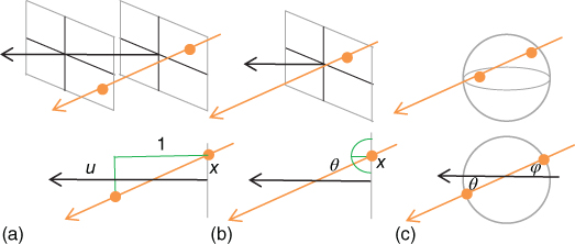
Figure 8.1 Light field parameterizations. (a) Two-plane parameterization, (b) spherical–Cartesian parameterization, and (c) sphere parameterization.

The light field can also be described in the frequency domain by means of its Fourier transform. Using the two-plane parameterization, we have

8.3

where are the spatial frequency variables and is the Fourier transform of the light field.

8.2.3 Light Field Reparameterization

When light traverses free space, the radiance along the light ray is unchanged, but the light field representation depends on the position of the reference planes. Different reference planes will be fixed to the optical elements of the plenoptic camera to study how rays change inside the camera body. Thus, the reference planes can be moved to arbitrary distance d or be coincident with the plane of a lens with focal length f.

If we displace the reference planes by d units, we can relate the original L₀ and new representation L₁ through a linear transform defined by a matrix . Similarly, we can describe the light field when light rays pass through a converging lens with focal length f aligning the spatial reference plane with the lens. In this case, we also obtain a linear transform defined by a matrix considering the thin lens model in Gaussian optics [9].

The matrix description of the transforms is shown below in the spatial and frequency domain using the two-plane parameterization with relative spatial coordinates (x, u) and relative frequency coordinates [10]:

8.4

8.5

Finally, it may be desirable to describe the light field by two reference planes separated by a distance B in absolute coordinates instead of the relative coordinates with unit distance separation. This is useful to parameterize the light field inside a camera where the spatial reference plane is aligned with the image sensor and the directional plane is aligned with the main lens. In this case, we can relate the original L₀ and new representation L₁ through a linear transform defined by a matrix :

8.6

where the scaling factor is the Jacobian of the transform. Since the transformations described above are linear, they can be combined to model more complex transforms simply by multiplying their associated matrices. Inverting the transform, it is also possible to describe the original light field L₀ in terms of the new representation L₁.

8.2.4 Image Formation

An image sensor integrates all the incoming radiances into a sensed irradiance value I(x):

8.7

Therefore, a conventional image is obtained integrating the light field with relative spatial coordinates along the directional u-axis. In Eq. (8.7), there is also an optical vignetting term. In the paraxial approximation [9], this term can be ignored. Geometrically, to obtain an image, we project the 2D light field into the spatial reference plane. In general case, for an n-dimensional signal, integration along n–kdimensions generates a k-dimensional image. For a 4D light field, we integrate along the 2D directional variables to obtain a 2D image. According to the slice theorem [11], projecting a signal in the spatial domain is equivalent to extracting the spectrum of a signal in the Fourier domain. This process is known as a slicing operation and can be described as

8.8

The advantage of this formulation is that integration in the spatial domain is replaced by taking the slice in the frequency domain that is a simpler operation.

8.2.5 Light Field Sampling

Light field recording devices necessarily capture a subset of the light field in terms of discrete samples. The discretization comes from two sources: the optical configuration of the device and the discrete pixels in the imaging sensor. The combined effect of these sources is to impose a specific geometry on the overall sampling of the light field. Understanding the geometry of the captured light field is essential to compare the different camera designs. In this section, we will explore different solutions to sample the light field and explore its properties.

8.2.5.1 Pinhole and Thin Lens Camera

The sampling geometry of an ideal pinhole camera is depicted in 2D in Figure 8.2. While this model treats pixels as having a finite spatial extent, the aperture is modeled as being infinitesimally small. The integration volume corresponding to each pixel of size Δp is a segment in the x-axis, taking on a value of zero everywhere except for u = 0. The sampling geometry of the thin lens model with an aperture of size Dis shown in Figure 8.3. Now, the integration volume for each pixel is a rectangle in the x, u plane, but as we can see from the sampling geometry, very low resolution is obtained in the directional reference plane u, so several approaches have been proposed to improve the directional resolution of the light field.

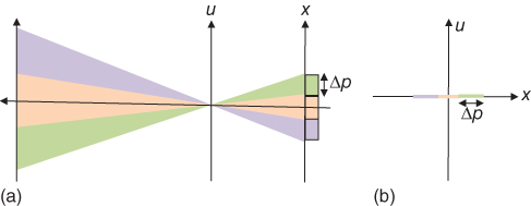
Figure 8.2 Pinhole camera. (a) Optical model and (b) light field representation.

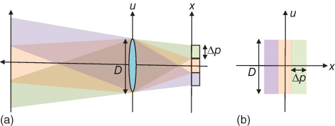
Figure 8.3 Thin lens camera. (a) Optical model and (b) light field representation. D is the lens aperture and Δp is the pixel size.

8.2.5.2 Multiple Devices

A straightforward approach to capture more information from the light field is the use of multiple devices. This is a solution also adopted in the biological domain that can be replicated with the use of an array of conventional 2D cameras distributed on a plane [12, 13]. If we adopt the pinhole approximation, sampling the light field from a set of images corresponds to inserting 2D slices into the 4D light field representation. Considering the image from each camera as a 2D slice of the 4D light field, an estimate of the light field is obtained from concatenating the captured slices. Camera arrays need geometric and color calibration and are expensive and complex to maintain, so there has been an effort to produce more manageable devices. In Figure 8.4, we show an example of a compact camera array composed of nine OV2640 cameras. The separation between them is 35 mm, the whole board is governed by a field programmable gate array (FPGA), and data transmission is performed through an Ethernet 1000 MB under UDP/IP. More compact arrays for mobile phones have also been developed [14].

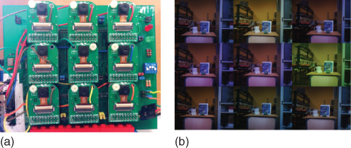
Figure 8.4 (a) A compact camera array. (b) Raw images from the array. Note the need for geometric and color calibration.

8.2.5.3 Temporal Multiplexing

Camera arrays cannot provide sufficient light field resolution in the directional dimension for several applications. This is a natural result of the camera size that physically limits the cameras from being located close to each other. To handle this limitation, the temporal multiplexing approach uses a single camera to capture multiple images from the camera array by moving its location [8, 15]. The position of the camera can be controlled precisely using a camera gantry or estimated from the captured images by structure from motion (SFM) algorithms. The disadvantages of the time-sequential capture include the difficulty of capturing dynamic environments and videos, its slowness because the position of the camera or the object has to be altered before each exposure, and the necessity of either gantry or the SFM algorithms to work in controlled environments.

8.2.5.4 Frequency Multiplexing

Temporal multiplexing solves some of the problems associated with camera arrays, but it has to be applied to static scenes, so other means of multiplexing the 4D light field into a 2D image are required to overcome this limitation. In Ref. [16], the frequency multiplexing approach is introduced as an alternative method to capture the light field using a single device. The frequency multiplexing method encodes different slices of the plenoptic function in different frequency bands and is implemented by placing nonrefractive light-attenuating masks in front of the image sensor. These masks provide frequency-domain multiplexing of the 4D Fourier transform of the light field into the Fourier transform of the 2D sensor image. The main limitation of these methods is that the attenuating mask limits the light entering in the camera.

8.2.5.5 Spatial Multiplexing

Spatial multiplexing produces an array of elemental images within the image captured with a single camera. This method began in the previous century with the works of Ives and Lippmann on integral imaging [[17, 18]]. Spatial multiplexing allows capturing dynamic scenes and videos but transfers spatial sampling resolution in favor of directional sampling resolution. One implementation of a spatial multiplexing system uses an array of microlenses placed near the image sensor. This device is called a plenoptic camera and will be described in Section 8.3. Examples of such implementations can be found in [3, 19–22].

8.2.5.6 Simulation

Light fields can also be obtained by rendering images from 3D models [23, 24]. By digitally moving the virtual cameras, this approach offers a low-cost acquisition method and easy access to several properties of the objects like their geometry or textures. It is also possible to simulate imperfections of the optical device or the sensor's noise behavior. Figure 8.5 shows an example of a simulated light field.

Figure 8.5 Simulated images from a light field.

8.2.6 Light Field Sampling Analysis

In the previous section, we reviewed several devices designed to sample the light field. If enough samples are taken from them, we expect to reconstruct the complete continuous light field. However, the light field is a 4D structure, so storage requirements are important and it is necessary to keep the samples to the minimum. The light field sampling problem is difficult because the sampling rate is determined by several factors, including the scene geometry, the texture on the scene surface, or the reflection properties of the scene surface. In Ref. [25], it was proposed to perform the light field sampling analysis applying the Fourier transform to the light field and then sampling it based on its spectrum for a camera array. Assuming constant depth, a Lambertian surface, and no occlusions, the light field in the spatial domain is composed of constant slope lines, and the Fourier spectrum of the light field is a slanted line. By considering all depths or equivalently all slanted lines, the maximum distance between the cameras was found to be

8.9

where B is the highest spatial frequency of the light field, z_min and z_max are the depth bounds of the scene geometry, and is the focal length of the cameras. A more detailed analysis can be found in Ref. [26], where non-Lambertian and nonuniform sampling are considered. Sampling analysis of the plenoptic camera will be detailed in Section 8.4.1.

8.2.7 Light Field Visualization

In order to understand the light field properties, it is useful to have some way of visualizing its structure. Since it is not possible to display a 4D signal in a 2D image, the 4D light field will be represented joining multiple 2D slices from the 4D signal to obtain a 2D multiplexed image. The directional information for a light field with relative spatial coordinates (x, y, u, v) can be visualized extracting a u, v slice of the light field fixing the spatial variables x and y. In Figure 8.6, we see all the u, v slices spatially multiplexed. Another alternative shown in Figure 8.7 is to fix a direction u, v and let the spatial variables x and y vary. These images can be interpreted as images from a camera array. Finally, in Figure 8.8, the pair of variables x and u (or y and v) are fixed and the other pair vary. The resulting images are called epipolar images of the light field. These epipolar images can be used to estimate the depth of the objects using the slope of the lines that compose them [27]. In a plenoptic camera, a line with zero slope indicates that the object is placed on the focus plane, while nonzero absolute values for slope indicate that the object is at a greater distance from the focus plane.

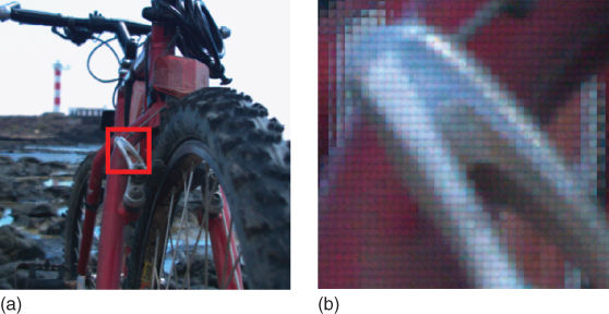
Figure 8.6 Fixing the spatial variables (x, y) and varying the directional variables (u, v) give the directional distribution of the light field. On (a), we see the 4D light field as a 2D multiplexed image. The image in (b) is a detail from (a). Each small square in (b) is the (u, v) slice for a fixed (x, y).

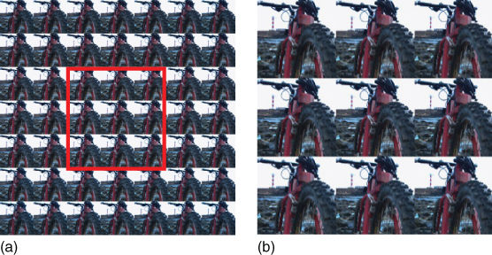
Figure 8.7 Fixing the directional variables (u, v) and varying the spatial variables (x, y) can be interpreted as taking images from a camera array. On (a), we see the 4D light field as another 2D multiplexed image. Image (b) is a detail from (a). Each image in (b) is the (x, y) slice for a fixed (u, v).

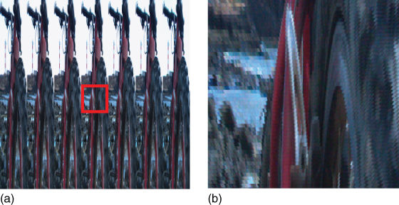
Figure 8.8 Fixing one-directional variable (u or v) and one spatial variable (x or y) generates another 2D multiplexed image. This is the epipolar image that gives information about the depth of the elements in the scene. On (b), we see a detail from (a). Note the different orientations corresponding to different depths in the scene.

8.3 The Plenoptic Camera

A plenoptic camera captures the 4D light field by placing a microlens array between the lens of the camera and the image sensor to measure the radiance and direction of all the light rays in a scene. The fundamental ideas behind the use of plenoptic cameras can be traced back to the beginning of the previous century with the works of Lippmann and Ives on integral photography [17, 18]. A problem of the Lippmann's method is the presence of pseudoscopic images (inverted parallax) when the object is formed at reconstruction. Different methods have been proposed for avoiding pseudoscopic images in real-time applications [28, 29]. One of the first plenoptic cameras based on the principles of integral photography was proposed in the computer vision field by Adelson and Wang [19] to infer depth from a single image. Other similar systems were built by Okano et al. [30] and Naemura et al. [31] using graded-index microlens arrays. Georgeiv et al. [32] have also used an integral camera composed of an array of lenses and prisms in front of the lens of an ordinary camera. Another integral imaging system is the Shack–Hartmann sensor [33] that is used to measure aberrations in optical systems. The plenoptic camera field experimented a great impulse when Ng [20] presented a portable handheld plenoptic camera. Its basic optical configuration comprises a photographic main lens, an N_x × N_x microlens array, and a photosensor array with N_u × N_u pixels behind each microlens. Figure 8.9 illustrates the layout of these components. Parameters D and d are the main lens and microlens apertures, respectively. Parameter B is the distance from the microlens x plane to the main lens u plane, and parameter b is the distance from the microlens plane to the sensor plane. Δp is the pixel size. The main lens may be translated along its optical axis to focus at a desired plane at distance A. As shown in Figure 8.9, rays of light from a single point on space converge on a single location in the plane of the microlens array. Then, the microlens at that location separates these light rays based on direction, creating a focused image of the main lens plane.

To maximize the directional resolution, the microlenses are focused on the plane of the main lens. This may seem to require a dynamic change of the separation between the photosensor plane and microlens array since the main lens moves during focusing and zooming. However, the microlenses are vanishingly small compared to the main lens, so independently of its zoom or focus settings, the main lens is fixed at the optical infinity of the microlenses by placing the photosensor plane at the microlenses' focal depth [19].

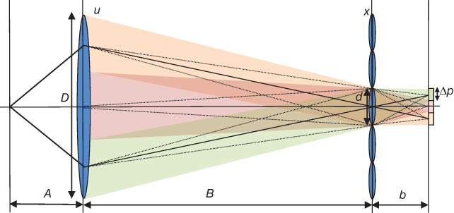
Figure 8.9 Optical configuration of the plenoptic camera (not shown at scale).

To describe the light rays inside the plenoptic camera, an initial light field L₀ is defined aligning a directional reference plane with the image sensor and a spatial reference plane with the microlens plane. We can describe in absolute coordinates the light field inside the camera L₁ after light rays pass through the microlens s of length d and focal length f aligning the same spatial reference plane with the microlens plane and a directional reference plane with the main lens plane. The relation between L₀ and L₁ can be described using the transforms in Section 8.2.3 as

8.10

where P is a permutation matrix that interchanges the components of a vector since rays in L₀ and L₁ point in a different direction.

Equation (8.10) can be explained as follows. We take a ray in light field L₁ defined from a point x on the microlens plane to a point u on the main lens plane and denote it by (x, u), and we want to obtain the corresponding ray (x, u′) defined from the microlens plane to the sensor plane as seen in Figure 8.10. To obtain (x, u′), we change the optical axis from the main lens to the microlens s of length d obtaining the ray (x–ds, u–ds) with coordinates relative to the new optical axis. As shown in Figure 8.10, the distance between the microlens plane and the main lens plane is B, so we use to rewrite (x–ds, u–ds) using a unit distance reference plane from the microlens plane in the main lens direction. Ray (x–ds, u–ds)^T passes through the microlens s with focal length f that changes its direction, so we use to obtain the transformed ray (x–ds, u–ds)^T defined from the microlens plane to the unit distance plane. To obtain the corresponding ray in L₀, we have to move both reference planes b units using to obtain the ray defined by (x–ds, u–ds)^T. Now, we separate the unit distance reference plane to distance b obtaining the ray (x–ds, u–ds)^T from the sensor plane to the microlens plane. Since we are interested that rays in L₀ point from the microlens plane to the sensor plane, we permute their coordinates using P. The final step is to move again the optical axis to the main lens axis obtaining the ray (x, u′)^T = (x–ds, u–ds)^T + (ds, ds)^T in L₀. The relation between the radiance of rays (x, u) in L₁ and (x, u′) in L₀ is defined in Eq. (8.10).

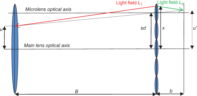
Figure 8.10 Ray transform in the plenoptic camera.

Computing the matrix products, Eq. (8.10) can be rewritten as

8.11

In order to use as many photosensor pixels as possible, it is desirable to choose the relative sizes of the main lens and microlens apertures so that the images under the microlenses are as large as possible without overlapping. Using Eq. (8.11), we see that the image of the main lens aperture in relative coordinates to microlens s is approximately since . To use the maximum extent of the image sensor, we must have the f-number condition since u varies within the aperture values . Note that the f-number condition is defined in terms of the image-side f-number, which is the diameter of the lens divided by the separation between the corresponding planes. Using Eq. (8.11), we can represent the sampling geometry of each pixel in L₁ as shown in Figure 8.11. Note the difference between the sampling pattern of Figures 8.3 and 8.10. In a plenoptic camera, the directional coordinate u is sampled, while in a conventional camera, the corresponding samples are integrated. Another result that can be seen from Figure 8.11 is that each row through the x-axis corresponds to an image taken from an aperture of size D/N_u. This implies that the depth of field of such images is extended N_u times relative to a conventional photograph.

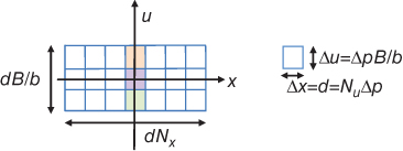
Figure 8.11 Sampling geometry of the plenoptic camera in L₁. Each vertical column corresponds to a microlens. Each square corresponds to a pixel of the image sensor.

The plenoptic model of this section represents a simplified representation of reality since it does not account for lens distortion or unwanted rotations between the microlens array and the photosensor plane. Therefore, a prior step to use this model in practical applications is to calibrate the plenoptic camera [34]. Images recorded from several plenoptic cameras can be obtained from [35–38].

8.4 Applications of the Plenoptic Camera

8.4.1 Refocusing

In conventional photography, the focus of the camera must be fixed before the shot is taken to ensure that selected elements in the scene are in focus. This is a result of all the light rays that reach an individual pixel being integrated as seen in Figure 8.3. With the plenoptic camera, the light field is sampled directionally, and the device provides the user with the ability to refocus images after the moment of exposure. If L₁ is a light field from the microlens plane to the main lens plane, the image is refocused by virtually moving the microlens plane to a distance Bα from the main lens plane obtaining a light field and applying the image formation operator in Eq. (8.7) as seen in Figure 8.12(b). For a 2D light field, we have

8.12

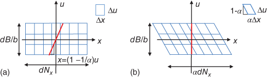
Figure 8.12 (a) Light field inside the camera. Refocusing is equivalent to integration along lines with x–u slope . (b) Equivalent light field with x–u slope after virtually moving the focusing plane.

Then, applying the image formation operator, we obtain

8.13

From Eq. (8.13), refocusing to a virtual plane is equivalent to integration along lines with slope . It can be interpreted as shifting for each u the subaperture image with an amount of and adding all the shifted subaperture images. If we assume that a plenoptic camera is composed of N_x × N_x microlenses and each microlens generates an N_u × N_u image with O(N_x) = O(N_u), then the full sensor resolution is O((N_x N_u)²) = O(N⁴). In this case, the shift and add approach needs O(N⁴) operations to generate a single photograph refocused on a determined distance.

A significant improvement to this performance was obtained in Ref. [20] with the Fourier slice photography technique that reformulates the problem in the frequency domain. This technique decreased the computational cost to O(N⁴log(N)) to generate a set of photographs with size O(N²), giving O(N²log(N)) operations to compute a O(N²) refocused image. This technique is based on the slicing operation in Eq. (8.8). Then, using Eq. (8.13), we obtain Eq. (8.14) indicating that a refocused photograph is a slanted slice in the Fourier transform of the light field. This can be seen graphically in Figure 8.13:

8.14

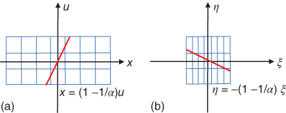
Figure 8.13 Fourier slice theorem. (a) Spatial integration. (b) Fourier slicing.

Then, in order to obtain a photograph, we have to compute first the Fourier transform of the light field . After that, we have to evaluate the slice , and finally, we have to compute the inverse Fourier transform of the slice. A discrete version of the Fourier slice theorem can be found in Ref. [39]. An example of the refocusing technique is shown in Figure 8.14. To characterize the performance of the refocusing process, it is necessary to obtain the range of depths for which we can compute an exact refocused photograph. If we assume a band-limited light field, the refocusing range is [20]

8.15

Figure 8.14 Image refocusing at several distances using the discrete focal stack transform [39].

In this slope interval, the reconstruction of the photograph from the samples of the light field is exact.

8.4.2 Perspective Shift

In addition to the refocusing capability of the plenoptic camera, it is also possible to view the scene from different perspectives, allowing the viewer a better angular knowledge of the world. As explained in Section 8.3, the pixels under each microlens collect light rays from a certain direction. Thus, considering the same pixel under each microlens, it is possible to compose a picture of the scene viewed from that direction. Perspective images are shown in Figure 8.7.

8.4.3 Depth Estimation

Plenoptic cameras can also provide 3D information about the scene indicating the depth of all pixels in the image [39, 40]. In fact, the plenoptic camera as a depth-sensing device is equivalent to a set of convergent cameras [41]. Based on this 3D information, it is also possible to obtain extended depth of field images in which all the elements in the image are in focus. In Figure 8.15, we show the basic geometry of depth estimation.

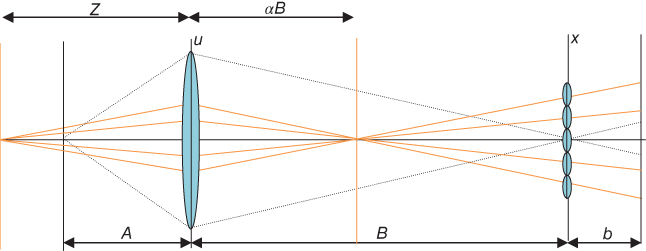
Figure 8.15 Geometry of depth estimation with a plenoptic camera.

It can be seen in the figure above that a Lambertian point at distance Z in the scene is transformed through the lens to a point at distance from the main lens. The set of rays emanating from this point is simply a line in 2D plenoptic space with equation . Then, we can obtain the depth of the point estimating the slope of the line in the epipolar image that was presented in Section 8.2.7. This approach is widely employed due to its simplicity [19, 42]. For example, we may write the light field L for all points (x_i, u_i) in a neighborhood N(x, u) of a point (x, u) as . Then, noting that in the direction , 1) the light field is constant due to the Lambertian assumption, we obtain the set of equations . Then, we can define a variance measure as the sum of the in the neighborhood N(x, u), and we can estimate the unknown slope through minimizing as [19]

8.16

8.17

Note that the estimation is unstable when the denominator is close to zero. This occurs in regions of the image with insufficient detail as is common in all passive depth recovery methods. Another alternative is to use a depth from focus approach. If we take a photograph of the Lambertian point at distance from the main lens with the sensor placed at a virtual distance of from the main lens, we obtain a constant element with radius

8.18

Then, we can obtain refocused images for several values of and select the sharpest one (the image with the smallest radius). There are several focus measures FM that can be employed which are basically contrast detectors within a small spatial window in the image. Unfortunately, the selection of the sharpest point is also unstable when the image has insufficient detail and some regularization method has to be employed to guide the solution. In Ref. [39], the Markov random field approach is used to obtain the optimal depth minimizing an energy function. Other regularization approaches include variational techniques [42]. Some examples of depth estimation are shown in Figure 8.16. In order to use the plenoptic camera as a depth recovery device, it is interesting to study its depth discrimination capabilities. This is defined as the smallest relative distance between two on-axis points, one at the focusing distance Z of the plenoptic camera and the other at Z′ which would give a slope connecting the central pixel of the central microlens with a border pixel of an adjacent microlens. The relative distance can be approximated as [43]

8.19

where d is the microlens size, k is the f-number of the camera, is the field of view, and S is the sensor size. Therefore, to increase the depth discrimination capabilities, it is necessary to select small values of the microlens size, f-number, field of view, and focusing distance and to select high values of the sensor size.

Figure 8.16 Depth estimation and extended depth of field images.

8.4.4 Extended Depth of Field Images

Another feature of plenoptic cameras is their capability to obtain extended depth of field images also known as all-in-focus images [3, 39]. The approach in light field photography is to capture a light field, obtain the refocused images at all depths, and select for each pixel the appropriate refocused images according to the estimated depth. Extended depth of field images is obtained in classical photography reducing the size of the lens aperture. An advantage of the plenoptic extended depth of field photograph is the use of light coming through a larger lens aperture allowing images with a higher signal to noise ratio. Examples of extended depth of field images are shown in Figure 8.16.

8.4.5 Superresolution

One of the major drawbacks of plenoptic cameras is that capturing a certain amount of directional resolution requires a proportional reduction in spatial resolution. If the number of microlenses is N_x × N_x and the pixels behind each microlens are N_u × N_u, the refocused images have a resolution of N_x × N_x and sensor resolution is reduced with a factor of (N_u)². Two approaches to increase the resolution can be found in plenoptic cameras. In this section, we will present some software-based methods, while in Section 8.5, hardware-based methods will be shown. Software-based superresolution methods discard the optimal sampling assumption of the light field of Section 8.4.1 and try to recover the light field using the aliased recorded plenoptic image. In Ref. [44], it is shown how to build superresolution refocused photographs that have a common size of approximately one-fourth of the full sensor resolution. It recovers the superresolution photograph, assuming that the scene is Lambertian and composed of several planes of constant depth. Since depth in the light field is unknown, it is estimated by the defocus method in Section 8.4.3. In Ref. [45], the superresolution problem was formulated in a variational Bayesian framework to include blur effects reporting a 7× magnification factor. In Ref. [46], the Fourier slice technique of [39] that was developed for photographs with standard resolution is extended to obtain superresolved images. Depth is also estimated by the defocus method in Section 8.4.3. In Figure 8.17, some results of the Fourier slice superresolution technique are shown.

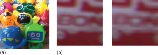
Figure 8.17 (a) Superresolution photographs from a plenoptic camera. (b) Comparison of superresolution (left) against bilinear interpolation (right).

8.5 Generalizations of the Plenoptic Camera

The previous section described a plenoptic camera where the microlenses are focused on the main lens. This is the case that provides a maximal directional resolution. The major drawback of the plenoptic camera is that capturing a certain amount of directional resolution requires a proportional reduction in the spatial resolution of the final photographs. In Ref. [3], a generalized plenoptic camera is introduced that provides a simple way to vary this trade-off, by simply reducing the separation between the microlenses and photosensor. This generalized plenoptic camera is also known as the focused plenoptic camera or plenoptic 2.0 camera [21]. To study the generalized plenoptic camera, β is defined to be the separation measured as a fraction of the depth that causes the microlenses to be focused on the main lens. For example, the standard plenoptic camera corresponds to β = 1, and the configuration where the microlenses are pushed against the photosensor corresponds to β = 0. A geometrical configuration of the generalized plenoptic camera is shown in Figure 8.18.

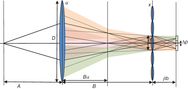
Figure 8.18 Geometry of a generalized plenoptic camera. Microlenses are now placed at distance βb from the sensor and focused on a plane at distance Bα from the main lens. Standard plenoptic camera corresponds to β = 1, α = 0.

As in Section 8.3, to describe the light rays inside the camera, a light field L₀ is defined aligning a directional reference plane with the image sensor and a spatial reference plane with the microlens plane. We also describe the light field inside the camera L₁ after light rays pass through the microlens s of length d aligning a spatial reference plane with the microlens plane and a directional reference plane with the main lens plane. The relation between L₀ and L₁ can be described as

8.20

That can be explicitly written as

8.21

Using Eq. (8.21), we can represent the sampling geometry of each pixel as shown in Figure 8.19(a). Note the difference between the sampling pattern of the standard plenoptic camera in Figure 8.11 and the generalized plenoptic camera. As the β value changes from 1, the light field sampling pattern shears within each microlens. This generates an increase in spatial resolution and a decrease in the directional resolution. If the resolution of the sensor is N_p × N_p and there are N_u × N_u pixels behind each of the N_x × N_x microlenses, the refocused images have a resolution of N_r × N_r, where

8.22

and the increment in resolution is ((1 − β) N_u)² that is (1 − β)² times the number of pixels in each microlens [3, 47]. Note that the change of pixel size in the x-axis is reflected in Figures 8.11 and 8.19 varying from d to Δp/(1 − β) leading to the increment in resolution in Eq. (8.22).

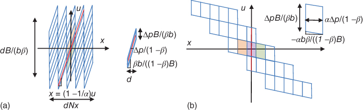
Figure 8.19 Sampling geometry of the generalized plenoptic camera. (a) Sampling in L₁. Each vertical column corresponds to a microlens. Each sheared square corresponds to a pixel of the image sensor. Pixel slope in the x–u plane is βb/((1 − β)B). (b) Sampling in L_r where the microlens plane is at distance Bα from the main lens and α verifies Eq. (8.23).

In order to exploit the resolution capabilities of the generalized plenoptic camera, the focus of its main lens has to be done differently than in a conventional or plenoptic camera [3]. In conventional and standard plenoptic cameras, best results are obtained by optically focusing on the subject of interest. On the other side, as shown in Figure 8.19(a), the highest final image resolution occurs when the refocusing plane verifies:

8.23

or equivalently . The sampling pattern for a light field Lr where the microlens plane is at distance Bα from the main lens plane and α verifies Eq. (8.23) is shown in Figure 8.19(b). If we want to obtain the maximum resolution at depth B, we should optically focus the main lens by positioning it at depth B/α for an optimal focusing distance of

8.24

Refocused photographs from a generalized plenoptic camera are shown in Figure 8.20. Other generalizations of the standard design include the use of microlenses with different focal lengths [48, 49] to increase the depth of field of the generalized plenoptic camera or the use microlenses with different apertures to obtain high-dynamic-range imaging [50].

Figure 8.20 Refocusing from a generalized plenoptic camera.

8.6 High-Performance Computing with Plenoptic Cameras

Processing and rendering the plenoptic images require significant computational power and memory bandwidth. At the same time, interactive rendering performance is highly desirable so that users can explore the variety of images that can be rendered from a single plenoptic image. For example, it is desirable to analyze the refocused photographs as a whole to estimate depth or to select a group of them with focus on determined elements. Therefore, it is convenient to use fast algorithms and appropriate hardware platform such as FPGA or graphics processing unit (GPU). A GPU is a coprocessor that takes on graphical calculations and transformations so that the main CPU does not have to be burdened by them. The FPGAs are semiconductor devices that are based on a matrix of configurable logic blocks connected via programmable interconnects. This technology makes possible to insert the applications on a custom-built integrated circuits. Also, FPGA devices offer extremely high-performance signal processing through parallelism and highly flexible interconnection possibilities. In Ref. [44], a method is presented for simultaneously recovering superresolved depth and all-in-focus images from a standard plenoptic camera in near real time using GPUs. In Ref. [51], a GPU-based approach for light field processing and rendering for a generalized plenoptic camera is detailed. The rendering performance allows to process 39 Mpixel plenoptic data to 2 Mpixel images with frame rates in excess of 500 fps. Another application example for FPGAs is presented in Ref. [52]. The authors describe a fast, specialized hardware implementation of a superresolution algorithm for plenoptic cameras. Results show a time reduction factor of 50 in comparison with the solution on a conventional computer. Another algorithm designed for FPGA devices is shown in Ref. [53]. The authors describe a low-cost embedded hardware architecture for real-time refocusing based on a standard plenoptic camera. The video output is transmitted via High-Definition Multimedia Interface (HDMI) with a resolution of 720p at a frame rate of 60 fps conforming to the HD-ready standard.

8.7 Conclusions

During the last years, the field of computational photography continued developing new devices with unconventional structures that extend the capabilities of current commercial cameras. The design of these sensors is guided toward increasing the information that can be captured from the environment. The available visual information can be described through the plenoptic function and its simplified 4D light field representation. In this chapter, we have reviewed several devices to capture this visual information and shown how the plenoptic camera captures the light field by inserting a microlens array between the lens of the camera and the image sensor measuring the radiance and direction of all the light rays in a scene. We have explained how the plenoptic images can be used, for instance, to change the scene viewpoint, to refocus the image, to estimate the scene depth, or to obtain extended depth of field images. The drawback of the plenoptic camera in terms of spatial resolution loss has also been detailed, and some solutions to overcome these problems have also been presented. Finally, we have explored the computational part of the techniques presented in high-performance computing platforms such as GPUs and FPGAs.

The plenoptic camera has left the research laboratories, and now, several commercial versions can be found [4, 5, 13]. We expect that the extension of its use will increase the capabilities of current imaging sensors and drive imaging science to new directions.

References

1. 1. Goldstein, E.B. (2009) Encyclopedia of Perception, SAGE Publications, Inc., Los Angeles, CA.

2. 2. Duparré, J.W. and Wippermann, F.C. (2006) Micro-optical artificial compound eyes. Bioinspir. Biomim., 1 (1), R1–16.

3. 3. Ng, R. (2006) Digital light field photography. PhD dissertation, Stanford University.

4. 4. Lytro. https://www.lytro.com (accessed 4 July 2014).

5. 5. Raytrix. http://www.raytrix.de/ (accessed 04 July 2014).

6. 6. Neumann, J., Fermuller, C., and Aloimonos, Y. (2003) Eye design in the plenoptic space of light rays. Proceedings of the Ninth IEEE International Conference on Computer Vision, Vol. 2, pp. 1160–1167.

7. 7. Adelson, E.H. and Bergen, J.R. (1991) The plenoptic function and the elements of early vision. Computational Models of Visual Processing, pp. 3–20.

8. 8. Levoy, M. and Hanrahan, P. (1996) Light field rendering. in Proceedings of the 23rd Annual Conference on Computer Graphics and Interactive Techniques, New York, pp. 31–42.

9. 9. Born, M. and Wolf, E. (1999) Principles of Optics, 7th edn, Cambridge University Press.

10.10. Liang, C.-K., Shih, Y.-C., and Chen, H.H. (2011) Light field analysis for modeling image formation. IEEE Trans. Image Process., 20 (2), 446–460.

11.11. Bracewell, R.N. (1990) Numerical transforms. Science, 248 (4956), 697–704.

12.12. Wilburn, B., Joshi, N., Vaish, V., Talvala, E.-V., Antunez, E., Barth, A.A., Adams, A., Horowitz, M., and Levoy, M. (2005) High performance imaging using large camera arrays. ACM SIGGRAPH 2005 Papers, New York, pp. 765–776.

13.13. Liu, Y., Dai, Q., and Xu, W. (2006) A real time interactive dynamic light field transmission system. 2006 IEEE International Conference on Multimedia and Expo, pp. 2173–2176.

14.14. Pelican Imaging. http://www.pelicanimaging.com/ (accessed 09 July 2014).

15.15. Gortler, S.J., Grzeszczuk, R., Szeliski, R., and Cohen, M.F. (1996) The lumigraph. Proceedings of the 23rd Annual Conference on Computer Graphics and Interactive Techniques, New York, pp. 43–54.

16.16. Veeraraghavan, A., Raskar, R., Agrawal, A., Mohan, A., and Tumblin, J. (2007) Dappled photography: mask enhanced cameras for heterodyned light fields and coded aperture refocusing. ACM SIGGRAPH 2007 Papers, New York.

17.17. Ives, F. (1903) Parallax stereogram and process of making same. US 725567.

18.18. Lippmann, G. (1908) Epreuves reversibles donnant la sensation du relief. J. Phys., 7 (4), 821–825.

19.19. Adelson, E.H. and Wang, J.Y.A. (1992) Single lens stereo with a plenoptic camera. IEEE Trans. Pattern Anal. Mach. Intell., 14 (2), 99–106.

20.20. Ng, R. (2005) Fourier slice photography. ACM SIGGRAPH 2005 Papers, New York, pp. 735–744.

21.21. Lumsdaine, A. and Georgiev, T. (2009) The focused plenoptic camera. 2009 IEEE International Conference on Computational Photography (ICCP), pp. 1–8.

22.22. Rodríguez-Ramos, J.M., Femenía Castellá, B., Pérez Nava, F., and Fumero, S. (2008) Wavefront and distance measurement using the CAFADIS camera. Proc. SPIE, Adaptive Optics Systems, 7015, 70155Q–70155Q–10.

23.23. Nava, F.P., Luke, J.P., Marichal-Hernandez, J.G., Rosa, F., and Rodriguez-Ramos, J.M. (2008) A simulator for the CAFADIS real time 3DTV camera. 3DTV Conference: The True Vision – Capture, Transmission and Display of 3D Video, pp. 321–324.

24.24. Wanner, S., Meister, S., and Goldluecke, B. (2013) Datasets and benchmarks for densely sampled 4D light fields. Vision, Modelling and Visualization (VMV).

25.25. Chai, J.-X., Tong, X., Chan, S.-C., and Shum, H.-Y. (2000) Plenoptic sampling. Proceedings of the 27th Annual Conference on Computer Graphics and Interactive Techniques, New York, pp. 307–318.

26.26. Zhang, C. and Chen, T. (2003) Spectral analysis for sampling image-based rendering data. IEEE Trans. Circuits Syst. Video Technol., 13 (11), 1038–1050.

27.27. Bolles, R.C., Baker, H.H., and Marimont, D.H. (1987) Epipolar plane image analysis: an approach to determining structure from motion. Int. Comp. Vis., 1, 1–7.

28.28. Arai, J., Kawai, H., and Okano, F. (2006) Microlens arrays for integral imaging system. Appl. Opt., 45 (36), 9066–9078.

29.29. Yeom, J., Hong, K., Jeong, Y., Jang, C., and Lee, B. (2014) Solution for pseudoscopic problem in integral imaging using phase-conjugated reconstruction of lens-array holographic optical elements. Opt. Express, 22 (11), 13659–13670.

30.30. Okano, F., Arai, J., Hoshino, H., and Yuyama, I. (1999) Three-dimensional video system based on integral photography. Opt. Eng., 38 (6), 1072–1077.

31.31. Naemura, T., Yoshida, T., and Harashima, H. (2001) 3-D computer graphics based on integral photography. Opt. Express, 8 (4), 255–262.

32.32. Georgeiv, T., Zheng, K.C., Curless, B., Salesin, D., Nayar, S., and Intwala, C. (2006) Spatio-angular resolution tradeoff in integral photography. Eurographics Symposium on Rendering, pp. 263–272.

33.33. Platt, B.C. and Shack, R. (2001) History and principles of Shack-Hartmann wavefront sensing. J. Refract. Surg. (Thorofare, NJ 1995), 17 (5), S573–577.

34.34. Dansereau, D.G., Pizarro, O., and Williams, S.B. (2013) Decoding, calibration and rectification for lenselet-based plenoptic cameras. 2013 IEEE Conference on Computer Vision and Pattern Recognition (CVPR), pp. 1027–1034.

35.35. Research – Raytrix GmbH. http://www.raytrix.de/index.php/Research.html (accessed 28 November 2014).

36.36. Plenoptic Imaging | ACFR Marine. http://www-personal.acfr.usyd.edu.au/ddan1654/LFSamplePack1-r2.zip (accessed 28 November 2014).

37.37. Heidelberg Collaboratory for Image Processing. http://hci.iwr.uni-heidelberg.de/HCI/Research/LightField/lf_benchmark.php (accessed 28 November 2014).

38.38. Todor Georgiev – Photoshop – Adobe. http://www.tgeorgiev.net/Gallery/ (accessed 28 November 2014).

39.39. Nava, F.P., Marichal-Hernández, J.G., and Rodríguez-Ramos, J.M. (2008) The discrete focal stack transform. Proceedings European Signal Processing Conference.

40.40. Tao, M.W., Hadap, S., Malik, J., and Ramamoorthi, R. (2013) Depth from combining defocus and correspondence using light-field cameras. IEEE International Conference on Computer Vision, Los Alamitos, CA, pp. 673–680.

41.41. Schechner, Y.Y. and Kiryati, N. (2000) Depth from defocus vs. stereo: how different really are they? Int. J. Comput. Vis., 39 (2), 141–162.

42.42. Wanner, S. and Goldluecke, B. (2014) Variational light field analysis for disparity estimation and super-resolution. IEEE Trans. Pattern Anal. Mach. Intell., 36 (3), 606–619.

43.43. Drazic, V. (2010) Optimal depth resolution in plenoptic imaging. 2010 IEEE International Conference on Multimedia and Expo (ICME), pp. 1588–1593.

44.44. Perez Nava, F. and Luke, J.P. (2009) Simultaneous estimation of super-resolved depth and all-in-focus images from a plenoptic camera. 3DTV Conference: The True Vision – Capture, Transmission and Display of 3D Video, pp. 1–4.

45.45. Bishop, T.E. and Favaro, P. (2012) The light field camera: extended depth of field, aliasing, and superresolution. IEEE Trans. Pattern Anal. Mach. Intell., 34 (5), 972–986.

46.46. Pérez, F., Pérez, A., Rodríguez, M., and Magdaleno, E. (2014) Super-resolved Fourier-slice refocusing in plenoptic cameras. J. Math. Imaging Vis., 52 (2), June 2015, 200–217.

47.47. Lumsdaine, A., Georgiev, T.G., and Chunev, G. (2012) Spatial analysis of discrete plenoptic sampling. Proc. SPIE, Digital Photography VIII, 8299, 829909–829909–10.

48.48. Perwass, C. and Wietzke, L. (2012) Single lens 3D-camera with extended depth-of-field. Proc. SPIE, Human Vision and Electronic Imaging XVII, 8291, 829108–829108–15.

49.49. Georgiev, T. and Lumsdaine, A. (2012) The multifocus plenoptic camera. Proc. SPIE, 8299, 829908–829908–11.

50.50. Georgiev, T.G., Lumsdaine, A., and Goma, S. (2009) High dynamic range image capture with plenoptic 2.0 camera. Frontiers in Optics 2009/Laser Science XXV/Fall 2009 OSA Optics & Photonics Technical Digest, p. SWA7P.

51.51. Lumsdaine, A., Chunev, G., and Georgiev, T. (2012) Plenoptic rendering with interactive performance using GPUs. Proc. SPIE, Image Processing: Algorithms and Systems X; and Parallel Processing for Imaging Applications II, 8295, 829513–829513–15.

52.52. Pérez, J., Magdaleno, E., Pérez Nava, F., Rodríguez, M., Hernández, D., and Corrales, J. (2014) Super-resolution in plenoptic cameras using FPGAs. Sensors, 14 (5), 8669–8685.

53.53. Hahne, C. and Aggoun, A. (2014) Embedded FIR filter design for real-time refocusing using a standard plenoptic video camera. Proc. SPIE, Digital Photography X, 9023, 902305.