Biologically Inspired Computer Vision (2015)

Part III
Modelling

Chapter 9
Probabilistic Inference and Bayesian Priors in Visual Perception

Grigorios Sotiropoulos and Peggy Seriès

9.1 Introduction

Throughout its life, an animal is faced with uncertainty about the external environment. There is often inherent ambiguity in the information entering the brain. In the case of vision, for example, the projection of a 3D physical stimulus onto the retina most often results in a loss of information about the true properties of the stimulus. Thus multiple physical stimuli can give rise to the same retinal image. For example, an object forming an elliptical pattern on the retina may indeed have an elliptical shape but it may also be a disc viewed with a slant (Figure 9.1). How does the visual system “choose” whether to see an ellipse or a slanted disc?

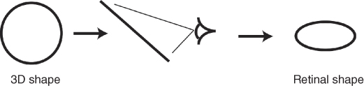
Figure 9.1 An elliptical pattern forming on the retina can be either an ellipse viewed upright or a circle viewed at an angle. Image adapted from Ref. [1] with permission.

Even in the absence of external ambiguity, internal neural noise or physical limitations of sensory organs, such as limitations in the optics of the eye or in retinal resolution, may also result in information loss and prevent the brain from perceiving details in the sensory input that are necessary to determine the structure of the environment.

Confronted with these types of uncertainty, the brain must somehow make a guess about the external world; that is, it has to estimate the identity, location, and other properties of the objects that generate the sensory input. This estimation may rely on sensory cues but also on assumptions, or expectations, about the external world. Perception has thus been characterized as a form of “unconscious inference” – a hypothesis first proposed by Hermann von Helmholtz (1821–1894). According to this view, vision is an instance of inverse inference whereby the visual system estimates the true properties of the physical environment from their 2D projections on the retina, that is, inverts the process of the mapping of the visual inputs onto the retina, with the help of expectations about the properties of the stimulus.

Helmholtz's view of perception as unconscious inference has seen a resurgence in popularity in recent years in the form of the “Bayesian brain” hypothesis [2–4]. In this chapter, we explain what it means to view visual perception as Bayesian inference. We review studies using this approach in human psychophysics. As we will see below, central to Bayesian inference is the notion of priors; we ask which priors are used in human visual perception and how they can be learned. Finally, we briefly address how Bayesian inference processes could be implemented in the brain, a question still open to debate.

9.2 Perception as Bayesian Inference

The “Bayesian brain hypothesis” proposes that the brain works by constantly forming hypotheses or “beliefs” about what is present in the world, and evaluates those hypotheses based on current evidence and prior knowledge. These hypotheses can be described mathematically as conditional probabilities: (Hypothesis |Data) is the probability of a hypothesis given the data (i.e., the signals available to our senses). These probabilities can be computed using Bayes' rule, named after Thomas Bayes (1701–1761):

9.1

Using Bayes' rule to update beliefs is called Bayesian inference. For example, suppose you are trying to figure out whether the moving shadow following you is that of a lion. The data available is the visual information that you can gather by looking behind you. Bayesian inference states that the best way to form this probability (Hypothesis | Data), called the posterior probability, is to multiply two other probabilities:

· (Data | Hypothesis): your knowledge about the probability of the data given the hypothesis (how probable is it that the visual image looks the way it does now when you actually know there is a lion?), which is called the likelihood, multiplied by:

· (Hypothesis) is the prior probability: our knowledge about the hypothesis before we could collect any information; here, for example, the probability that we may actually encounter a lion in our environment, independently of the visual inputs, a number which would be very different if we lived in Edinburgh rather than in Tanzania.

The denominator, (Data), is only there to ensure the resulting probability is between 0 and 1 and can often be disregarded in the computations. The hypothesis can be about the presence of an object, as in the example above, or about the value of a given stimulus (e.g., “the speed of this lion is 40 km/h” – an estimation task) or anything more complex.

Bayesian inference as a model of how the brain works thus rests on critical assumptions that can be tested experimentally:

· The brain takes into account uncertainty and ambiguity by always keeping track of the probabilities of the different possible interpretations.

· The brain has built (presumably through development and experience) an internal model of the world in the form of prior beliefs and likelihoods that can be consulted to interpret new situations.

· The brain combines new evidence with prior beliefs in a principled way, through the application of Bayes' rule.

An observer who uses Bayesian inference is called an ideal observer.

9.2.1 Deciding on a Single Percept

The posterior probability distribution obtained through Bayes' rule contains all the necessary information to make inferences about the hypothesis, , by assigning a probability to each value of . For example, the probability that we are being followed by a lion would be 10% and that there is no lion, 90%. But we only perceive one interpretation at a time (no lion), not a mixture of the two interpretations (90% lion and 10% no lion). How does the brain choose a single value of , based on the posterior distribution? This is not clearly understood yet but Bayesian decision theory provides a framework for answering this question. If the goal of the animal is to have the fewest possible mismatches between perception and reality, the value of that achieves this (call it should simply be the most probable value. This is called the maximum a posteriori (MAP) solution:

9.2

where denotes the data. Another possibility is to use the mean of the posterior (which is generally different to the maximum for skewed or multimodal distributions). This solution minimizes the squared difference of the inferred and actual percept, .

Taking either the maximum or the mean of the posterior is a deterministic solution: for a given posterior, this will lead to a solution that is always the same. In perceptual experiments, however, there is very often trial-to-trial variability in subjects' responses. The origin of this variability is debated.

One way to account for it with a Bayesian model is to assume that perception and/or responses are corrupted by noise. Two types of noise can be included: (i) perceptual noise in the image itself or in the neural activity of the visual system and (ii) decision noise – an additional source of noise between perception and response – for example, neural noise in motor areas of the brain that introduces variability in reporting what was seen, even when the percept itself is noiseless.

Another way to model trial-to-trial variability is to assume a stochastic rule for choosing . The most popular approach is probability matching, whereby is simply a sample from the posterior. Thus across trials, the relative frequency of a particular percept is equal to its posterior probability. It can be shown that probability matching is not an optimal strategy under the standard loss criteria discussed above. However, the optimality of a decision rule based on the maximum or the mean of the posterior rests on the assumption that the posterior is correct and that the environment is static; when either of theseis not true, probability matching can be more useful because it increases exploratory behavior and provides opportunity for learning. Probability matching and generally posterior sampling has also been proposed as a mechanism to explain multistable perception [5], whereby an ambiguous image results in two (or more) interpretations that spontaneously alternate in time. For example, looking at Figure 9.2, we might see a vase at one time but two opposing faces at another time. It has been proposed that such bistable perception results from sampling from a posterior distribution which would be bimodal, with two peaks corresponding to the two possible interpretations.

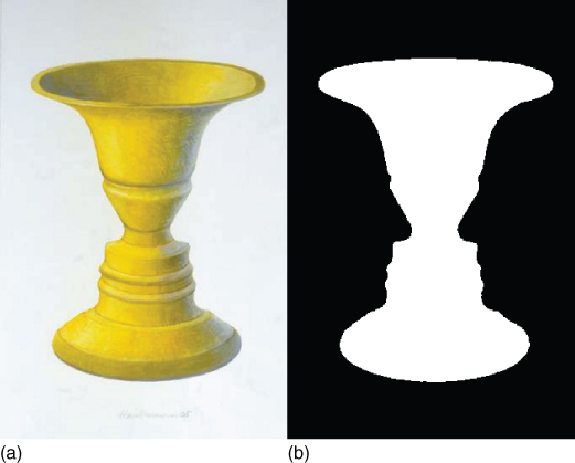
Figure 9.2 Rubin's vase. The black-and-white image (b) can be seen as a white vase or as two opposing black faces. The image (a) provide the context that primes the visual system to choose one of the interpretations for the ambiguous image: the vase, before it switches to the faces.

9.3 Perceptual Priors

As described above, the Bayesian brain hypothesis proposes that a priori knowledge is used in the perceptual inference and represented as a prior probability. Recently, a number of researchers have explored this idea: if the brain uses prior beliefs, what are those? And how do they influence perception?

Intuitively, it is when sensory data is limited or ambiguous that we rely on our prior knowledge. For example, if we wake up in the middle of the night and need to walk in total darkness, we automatically use our prior knowledge of the environment, or of similar environments, to guide our path. Mathematically, Bayes' rule similarly indicates that prior distributions should have maximum impact in situations of strong uncertainty. Thus, a good way to discover the brain's prior expectations is to study perception or cognition in situations where the current sensory inputs (the “evidence”) is limited or ambiguous. Studying such situations reveals that our brain uses automatic expectations all the time.

9.3.1 Types of Prior Expectations

Visual illusions are a great example of this. Consider Figure 9.2, for example. The ambiguous “Rubin's vase” can be interpreted as either a vase, or two faces facing each other. However, in Figure 9.2, because of the spatial proximity of the ambiguous image on the right with the photo of the vase (a), you are more likely to perceive first a vase (b), which will then switch to a face. The same effect would be observed with temporal proximity, such as when Rubin's vase is presented shortly after the unambiguous image of a vase. These types of expectations, induced by cues that are local in space or time and have immediate and short-term effects, have been recently dubbed “contextual expectations” [6]. There are several different types of contextual expectations that affect perception. Some experiments manipulate expectations by explicitly giving information regarding the visual stimulus, for example, telling participants about the number of possible directions of motion that they are going to be exposed to. In yet other psychophysical experiments, expectations are formed implicitly and unconsciously, for example, by exposing participants to the association between the sense of rotation of a 3D cylinder and a particular signal, for example a sound [7]. When the sense of rotation is later made ambiguous by removing 3D information, the subjects' perception will be modulated by the presence of the sound.

Contextual expectations are not the only kind of expectations; another kind, conceptually more akin to Bayesian priors, are expectations based on general, or prior, knowledge about the world. These have been referred to as structural expectations [6, 8]. The expectation that shapes are commonly isotropic is one such example: when humans see an elliptical pattern such as that of Figure 9.1, they commonly assume that it is a circle viewed at a slant rather than an ellipse because circles, being isotropic, are considered more common than ellipses. Another well-known effect is that the human visual system is more sensitive to cardinal (horizontal and vertical) orientations, the so-called “oblique effect.” This is thought to be due to an intrinsic expectation that cardinal orientations are more likely to occur than oblique orientations (see below). Another well-studied example of a structural expectation that has been formalized in Bayesian terms is that light comes from above us. The light-from-above prior is used by humans as well as other animals when inferring the properties of an object from its apparent shading. Figure 9.3(a), for example, is interpreted as one dimple in the middle of bumps. This is consistent with assuming that light comes from the top of the image. Turning the page upside down would lead to the opposite percept. In shape-from-shading judgments, as well as in figure–ground separation tasks, another expectation also influences perception—that objects tend to be convex rather than concave. For example, Figure 9.3(b) is typically interpreted as a set of black objects in white background (and not vice versa) because under this interpretation the objects are convex. A convexity prior seems to exist not just for objects within a scene (e.g., bumps on a surface) but also for the entire surface itself: subjects are better at local shape discrimination when the surface is globally convex rather than concave. A related, recently reported expectation is that depth (i.e., the distance between figure and ground) is greater when the figure is convex rather than concave. Other examples of expectations are that objects tend to be viewed from above; that objects are at a distance of 2–4 m from ourselves; that objects in nearby radial directions are at the same distance from ourselves; and that people's gaze is directed toward us (see [6] and citations therein). Finally, an expectation that has lead to numerous studies is the expectation that objects in the world tend to move slowly or to be still. In Bayesian models of motion perception, this is typically referred to as the slow speed prior (see below).

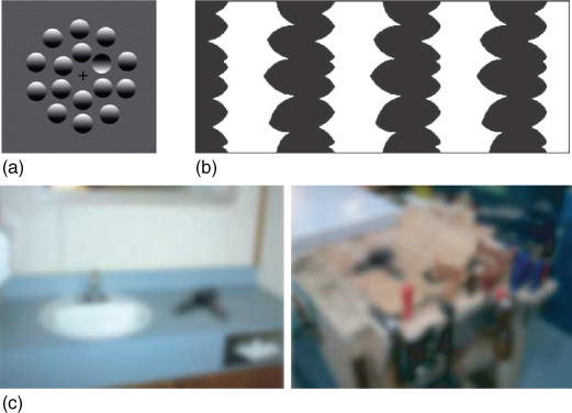
Figure 9.3 (a) Expectation that light comes from above. This image is interpreted as one dimple in the middle of bumps. This is consistent with assuming that light comes from the top of the image. Turning the page upside down would lead to the opposite percept. Image adapted from Ref. [9] with permission. (b) Convexity expectation for figure–ground separation. Black regions are most often seen as convex objects in a white background instead of white regions being seen as concave objects in a black background. Image adapted from Ref. [10] with permission. Interplay between contextual and structural expectations. The black object in (c) is typically perceived as a hair dryer because although it has a pistol-like shape (structural expectation), it appears to be in a bathroom (contextual expectation) and we know that hair dryers are typically found in bathrooms (structural expectation). The identical-looking black object in (d) is perceived as a drill because the context implies that the scene is a workshop. Image adapted from Ref. [11] with permission.

The distinction between contextual and structural expectations is not always clear-cut. For example, when you see a dark, pistol-shaped object in the bathroom after you have taken off your glasses and your vision is blurred, you will likely see that object as a hairdryer (Figure 9.3(c)). The exact same shape seen in a workshop will evoke the perception of a drill. The context, bathroom sink versus workbench, helps disambiguate the object – a contextual expectation. However, this disambiguation relies on prior knowledge that hair dryers are more common in bathrooms and drills are more common in workshops; these are structural expectations. In a Bayesian context, structural expectations are commonly described in terms of “priors.”

9.3.2 Impact of Expectations

Expectations help us infer the state of the environment in the face of uncertainty. In the “bathroom sink versus workbench” example, expectations help disambiguate the dark object in the middle of each image in Figure 9.3. Apart from aiding with object identification or shape judgments, expectations can impact perception in several other ways. First, they can lead to an improvement in performances during detection tasks. For example, when either the speed or the direction of motion of a random-dot stimulus are expected, subjects are better and faster at detecting the presence of the stimulus in a two-interval forced choice task [12]. More interestingly perhaps, in some cases, expectations about a particular measurable property can also influence the perceived magnitude of that property, that is, the content of perception. A recent study, forexample, showed that, when placed in a visual environment where some motion directions are more frequently presented than others, participants quickly and implicitly learn to expect those. These expectations affect their visual detection performance (they become better at detecting the expected directions at very low contrast) as well as their estimation performances (they show strong estimation biases, perceiving motion directions as being more similar to the expected directions). Moreover, in situations where nothing is shown, participants sometimes incorrectly report perceiving the expected motion directions – of the form of “hallucinations” of the prior distribution [13].

Another particularly interesting example of how expectations can affect the content of perception is the aforementioned expectation of slow speeds which we describe in more detail in the next section.

9.3.3 The Slow Speed Prior

Hans Wallach observed that a line moving behind a circular aperture, with its endpoints concealed such that its true direction cannot be recovered, always appears to move perpendicularly to its orientation [14]. This is known as the “aperture problem.” Observing that the perpendicular direction corresponds to the interpretation of the retinal image sequence which has slowest speed, he hypothesized that the reason for this remarkably universal perception is an innate preference of the visual system for slow speeds. This idea has been formalized by Weiss et al. in 2002 [15]. These researchers showed that a Bayesian model incorporating a prior for slow speeds can explain not only the aperture problem but also a variety of perceptual phenomena, including a number of visual illusions and biases.

One effect that this model explains is the “Thompson effect”—the decrease in perceived speed of a moving stimulus when its contrast decreases [16]. In the model of Weiss et al., the speed of a rigidly translating stimulus is determined by the integration of local motion signals under the assumptions of measurement noise and a prior that favors slow speeds. Given the noisy nature of eye optics and of neural activity, at low contrasts, the signal-to-noise ratio is lower than it is at high contrasts. This means that the speed measurements that the visual system performs are more noisy, which is reflected by a broader likelihood function. According to Bayes' rule, the prior will thus have a greater influence on the posterior at low contrasts than at high contrasts, where the likelihood is sharper. It follows that perceived speed will be lower at low contrasts (see Figure 9.4). A real-world manifestation of the Thompson effect is the well-documented fact that drivers speed up in the fog [18]. It should be noted that contrast is not the only factor that can affect uncertainty: similar biases toward slow speeds can be observed when the duration of the stimulus is shortened [19].

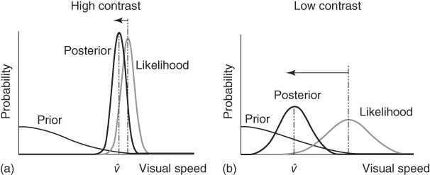
Figure 9.4 Influence of image contrast on the estimation of speed. (a) At high contrast, the measurements of the stimulus are precise, and thus lead to a sharp likelihood. Multiplication of the likelihood by the prior distribution leads to a posterior distribution that is similar to the likelihood, only slightly shifted toward the prior distribution. (b) At low contrast, on the other hand, the measurements are noisy and lead to a broad likelihood. Multiplication of the prior by the likelihood thus leads to a greater shift of the posterior distribution toward the prior distribution. This will result in an underestimation of speed at low contrast. Reproduced from Ref. [17] with permission.

The slow speed prior affects not only the perceived speed but also the perceived direction. The model of Weiss et al. accounts for the aperture problem as well as the directional biases observed with the motion of lines that are unoccluded but are presented at very low contrast. The rhombus illusion is a spectacular illustration of this. In this illusion (Figure 9.5), a thin, low-contrast rhombus that moves horizontally appears to move diagonally, whereas the same rhombus at a high contrast appears to move in its true direction. This illusion is well accounted by the model. Weiss et al. make a convincing case that visual illusions might thus be due not to the limitations of a collection of imperfect hacks that the brain would use, as commonly thought, but would be instead “a result of a coherent computational strategy that is optimal under reasonable assumptions.” See also Chapter 12 of this book for related probabilistic approaches to motion perception.

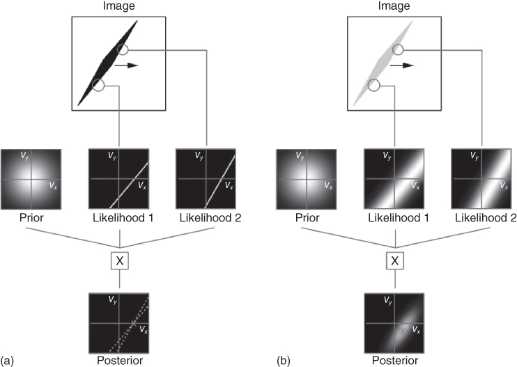
Figure 9.5 Influence of contrast on the perceived direction of a horizontally moving rhombus. (a). With a high-contrast rhombus the signal-to-noise ratio of the two local measurements (only two are shown for clarity) is high and thus the likelihood for each measurement in velocity space is sharp, tightly concentrated around a straight line, and dominates the prior, which is broader. The resulting posterior is thus mostly dictated by the combination of the likelihoods and favors the veridical direction (because the point where the two likelihood lines intersect has ). (b) With a low-contrast rhombus, the constraint line of the likelihood is fuzzy, that is, the likelihood is broad and the prior exerts greater influence on the posterior, resulting in a posterior that favors an oblique direction. Image adapted from Ref. [15], with permission.

9.3.4 Expectations and Environmental Statistics

If our perceptual systems are to perform well, that is, if the interpretation of an ambiguous or noisy scene is to match the real world as closely as possible, our expectations need to accurately reflect the structure of the real world. In Bayesian terms, this means that our priors must closely approximate the statistics of the environment (see Chapter 4 of this book). Using the previous “bathroom sink versus workbench” example, we need to have a prior that favors the presence of drills in workshops. If that were not the case, we might interpret the object in the workshop as a hair dryer, which would lead to an incorrect inference more often than not because, statistically speaking, drills are more common in workshops than hair dryers are.

Our visual input—the images forming on the retina—although very varied, is only a small subset of the entire possible image space. Natural images are highly redundant, containing many statistical regularities that the visual system may exploit to make inferences about the world. If expectations are to facilitate vision, they should approximate environmental statistics and, indeed, there is considerable evidence that in many cases they do so. For example, as described above, it is known that, when assessing the orientation of visual lines, human participants show strong biases toward cardinal orientations (vertical and horizontal), indicating a tendency to expect cardinal orientations in the world. Moreover, this bias is known to depend on the uncertainty associated with the stimulus [20]. This expectation is consistent with natural scene statistics : FFT analysis, for example, shows stronger power at cardinal compared with oblique orientations in a variety of natural images [21, 22]. The link between natural images statistics and the use of Bayesian priors in behavioral tasks was demonstrated recently by Girshick et al. [23]. Girshick et al. studied the performances of participants comparing different orientations, and found that participants were strongly biased toward the cardinal axes when the stimuli were uncertain. They further measured the distribution of local orientations in a collection of photographs and found that it was strongly nonuniform, with a dominance of cardinal directions. Assuming that participants behaved as Bayesian observers, and using a methodology developed by Stocker and Simoncelli [17], they could extract the Bayesian priors that participants used in the discrimination task and found that the recovered priors matched the measured environmental distribution (Figure 9.6).

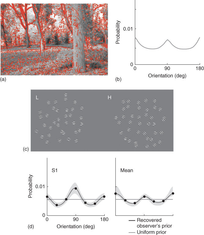
Figure 9.6 Expectations about visual orientations. (a) Example of a natural scene, with strongly oriented locations marked in red. (b) Distribution of orientations in natural scene photographs. (c) Participants viewed arrays of oriented Gabor functions and had to indicate whether the right stimulus was oriented counterclockwise or clockwise relative to the left stimulus. (d). The recovered priors, extracted from participants' performances, here shown for subject S1 and mean subject, are found to match the statistics of orientation in the natural scenes. Reproduced from Ref. [23] with permission.

Similarly, a study measured the pairwise statistics of edge elements from contours found in natural images and found that the way humans group edge elements of occluded contours matches the performance of an ideal observer Bayesian model, that is, a model with a prior reflecting the statistics of the natural image database [24]. This suggests that perceptual mechanisms of contour grouping are closely related to natural image statistics. The influence of the convexity expectation in figure–ground separation may also have a basis in natural scene statistics. As mentioned above, it was found that subjects expect greater distances between convex figures and background than between concave ones and background [25]. These expectations were in accord with the statistics of a collection of luminance and range images obtained from indoor and outdoor scenes.

As far as the slow speed prior is concerned, research related to the statistical structure of time-varying images is scarce. Inferring a distribution of object speeds from image sequences is complicated by the fact that retinal motion (the motion of patterns forming on the retina) does not correspond to object motion in a trivial way. One problem is that object speed can be inferred from retinal speed (the rate of movement of an object's projection on the retina) only if the distance of the object from the observer is known. Another problem is that retinal motion can be produced both by the independent motion of objects in the view field and by self-motion, head and eye movements. There are however some indications from studies looking at the properties of optical flow and the power spectrum of video clips that the distribution of retinal speeds can be described by a log-normal distribution or a power-law distribution favoring slow speeds [26, 27].

9.4 Outstanding Questions

While expectations have been studied for more than a century, the formalization of expectations as priors in Bayesian models of perception is relatively recent. Although by now there is a considerable body of theoretical work on Bayesian models that account for a wealth of perceptual data from human and nonhuman observers, there are a number of outstanding questions.

9.4.1 Are Long-Term Priors Plastic?

Are long-term priors hard-wired, or fixed after long-term exposure, or are they constantly updating through experience? This question was first addressed in the context of the light-from-above prior. In 1970, Hershberger showed that chickens reared in an environment illuminated from below did not differ from controls in their interpretation of shadows and depth [28]. They thus suggested that the prior thatlight comes from above is innate. This question was recently revisited in humans [29]. In their experiment, the authors first asked participants to make convex–concave judgments of bump–dimple stimuli at different orientations, and measured the light-from-above prior based on their responses. During a training phase, they then added new shape information via haptic (active touch) feedback, that disambiguated object shape but conflicted with the participants' initial interpretation, by corresponding to a light source shifted by 30 ° compared to the participants' baseline prior. When participants were finally tested again on visual only stimuli, their light direction prior had shifted significantly in the direction of the information provided during training. Adams et al. thus concluded that, unlike in chickens, the light-from-above prior could be updated in humans. We recently investigated this question in the context of the slow speed prior [30]. The aim of this study was to test whether expectations about the speed of visual stimuli could be implicitly changed solely through exposure to fast speeds and if so, whether this could result in a disappearance or reversal of the classically reported direction biases. Using a field of coherently moving lines presented at low contrast and short durations, this was found to be the case. After about hour exposure to fast speeds on three consecutive days, directional biases disappeared and a few days later, they changed sign, becoming compatible with a speed prior centered on speeds faster than 0 deg/s.

9.4.2 How Specific are Priors?

Another crucial issue that needs to be clarified concerns the specificity of expectations. For example, is there only one speed prior, which is applied to all types of visual objects and stimuli? Or are there multiple priors specific to different objects and conditions? When new priors are learned in the context of a task, do they automatically transfer to different tasks? Adams et al. provided evidence that the visual system uses the same prior about light source position in quite different tasks, one involving shape and another requiring lightness judgments [29]. Similarly, Adams measured the light-from-above in different tasks: visual search, shape perception, and a novel reflectance-judgment task [9]. She found strong positive correlations between the light priors measured using all three tasks, suggesting a single mechanism used for “quick and dirty” visual search behavior, shape perception, and reflectance judgments. In the context of short-term statistical learning, and using a familiarization task with complex shapes, Turk-Browne and Scholl (2009) provided evidence for transfer of perceptual learning across space and time, suggesting that statistical learning leads to flexible representations [31]. However, the generality of these findings is still unclear and needs further exploration. A related question is to understand whether expectations learned in the laboratory can persist over time and for how long. Recent work suggests that contextual priors persist over time, but may remain context-dependent, with the experimental setup acting as a contextual cue [32].

9.4.3 Inference in Biological and Computer Vision

The Bayesian approach is not the first computational framework to describe vision, whether artificial or biological, in terms of inverse inference. In a series of landmark papers published in the 1980s, Tomaso Poggio and colleagues postulated that inverse inference in vision is an ill-posed problem [33]. The term “ill-posed” was first used in the field of partial differential equations several decades earlier to describe a problem that has either multiple solutions, no solution, or the solution does not depend continuously on the data. Poggio and colleagues suggested that to solve the problem of inverse inference, the class of admissible solutions must be restricted by introducing suitable a priori knowledge. The concept of a priori knowledge, or assumptions, had been used earlier by Tikhonov and Arsenin [34] as a general approach to solving ill-posed problems in the form of regularization theory. Let be the data available and let be the stimulus of interest, such that , where is a known operator. The direct problem is to determine from ; the inverse problem is to obtain when is given. In vision, most problems are ill-posed because is typically not unique. Regularization works by restricting the space of solutions by adding the stabilizing functional, or constraint, . The solution is then found using

9.3

where is the estimate of the stimulus property (or properties) of interest; and is a constant that controls the relative weight given to the error in estimation versus the violation of the constraints when computing the solution. Thus approximates the inverse mapping under the constraints .

Since the work of Poggio and colleagues, regularization has been widely used in the computer vision community for a variety of problems, such as edge detection, optical flow (velocity field estimation), and shape from shading. These endeavors were met with success in many hard problems in vision—particularly problems that were hard to solve when the visual input were natural scenes rather than simplified artificial ones. This success lent popularity to the hypothesis, also central to the Bayesian approach, that the brain perceives the world by constraining the possible inverse inference solutions based on prior assumptions about the structure of the world. Bayesian inference and regularization have more in common than just this common concept, however. This becomes more apparent by taking the logarithm of the posterior in Bayes' rule equation (9.1):

The MAP solution of the log-posterior (which is the same as the MAP of the posterior, as logarithms are monotonic functions) thus becomes

9.4

where can been ignored as it does not depend on , and is expressed in terms of minimizing the sum of negative logarithms (instead of maximizing the sum of positive logarithms). The similarities between Eqs. (9.3) and (9.4) are striking: in both equations, the solution is derived by minimizing the sum of two quantities: one that is based on a forward-inference model and another that is proportional to the deviation of the solution from the one expected by prior knowledge/constraints. Bayesian inference can thus be regarded as a stochastic version of regularization — the main difference being that Bayesian inference is a more general and powerful framework. This is due to two reasons. First, Bayesian inference, being a probabilistic estimation theory, provides the optimal way of dealing with noise in the data ( in our case), whereas regularization can be sensitive to noise. Second, in Bayesian inference, the posterior also represents the reliability of each possible solution (whereas regularization is akin to only representing the mode of a posterior). In other words, a Bayesian approach makes use of all available information in situations of uncertainty (such as noisy measurements) and evaluates the relative “goodness” of each possible solution, as opposed to merely yielding the best solution.

Probabilistic approaches have been used in a number of ways in computer vision. They typically consist of graphical models, whereby different levels of representation of visual features are linked to each other as nodes in a graph. Particle filtering and Markov chain Monte Carlo [35] are two examples of techniques whereby a probability distribution (rather than a single value) of a property is maintained and used in subsequent computations (e.g., as more data is received). An example use of such techniques in computer vision is the CONDENSATION algorithm, a particle filtering approach for the tracking of dynamic, changing objects. Interestingly, electrophysiological data from neurons in early visual areas (such as V1) has revealed long latencies of responses, an indication that there are multiple levels of information processing where low (early) levels interact with higher ones. Some authors have suggested that these interactions can be modeled with the algorithms of particle filtering and Bayesian belief propagation [36].

Prior assumptions in graphical models are most often modeled with Markov random fields (MRF), which capture dependencies between neighboring elements in an image (such as collinearity between adjacent line elements) and are flexible enough to allow the specification of various types of prior knowledge.

As a final note, although Bayesian inference is a more general framework than regularization, it is also more costly in computational resources. Furthermore, many problems in vision can be solved without the need for a full probabilistic approach such as Bayesian inference. Thus Bayesian inference is not always used in computer vision and may not always be used in biological vision either — or may be used in an approximate manner [37, 38], for example, through the representation of approximate, simpler versions of the true likelihood and prior distributions.

9.4.4 Conclusions

Bayesian models and probabilistic approaches have been increasingly popular in the machine vision literature [39]. At the same time, they appear to be very useful for describing human perception and behavior at the computational level. How these algorithms are implemented in the brain and relate to neural activity is still an open question and an active area of research.

While its popularity has been steadily increasing in recent years, the Bayesian approach has also received strong criticism. Whether the Bayesian approach can actually make predictions for neurobiology, for example, on which parts of the brain would be involved, or how neural activity could represent probabilities, is debated. It is yet unclear whether the Bayesian approach is only useful at the “computational level,” to describe the computations performed by the brain overall, or whether it can be also useful at the “implementation level” to predict how those algorithms might be implemented in the neural tissue [40]. It has also been argued that the Bayesian framework is so general that it is difficult to falsify.

However, a number of models have been proposed that suggest how (approximate) Bayesian inference could be implemented in the neural substrate [36, 41]. Similarly, a number of suggestions have been made about how visual priors could be implemented. Priors could correspond to different aspects of brain organization and neural plasticity. Contextual priors could be found in the numerous feedback loops present in the cortex at all levels of the cortical hierarchy [36]. A natural way in which structural priors could be represented in the brain is in the selectivity of the neurons and the inhomogeneity of their preferred features: the neurons that are activated by the expected features of the environment would be present in larger numbers or be more strongly connected to higher processing stages than neurons representing non-expected features. For example, as discussed above, a Bayesian model with a prior on vertical and horizontal orientations (reflecting the fact that they are more frequent in the visual environment) can account for the observed perceptual biases toward cardinal orientations. These effects can also be simply accounted for in a model of the visual cortex where more neurons are sensitive to vertical and horizontal orientations than to other orientations. Another very interesting idea that has recently attracted much interest is that spontaneous activity in sensory cortex could also serve to implement prior distributions. It is very well known that the brain is characterized by ongoing activity, even in the absence of sensory stimulation. Spontaneous activity has been traditionally considered as being just “noise.” However, the reason the brain is constantly active might be because it continuously generates predictions about the sensory inputs, based on its expectations. This would be computationally advantageous, driving the network closer to states that correspond to likely inputs, and thus shortening the reaction time of the system.

Finally, a promising line of work is interested in relating potential deficits in Bayesian inference with psychiatric disorders [42]. It is well known that the visual experience of patients suffering from mental disorders such as schizophrenia and autism are different from that of healthy controls. Recently, such differences have been tentatively explained in terms of differences in the inference process, in particular regarding the influence of the prior distributions compared to the likelihood. For example, priors that would be too strong could lead to hallucinations (such as in schizophrenia), while priors that would be too weak could lead to patients being less susceptible to visual illusions, and to the feeling of being overwhelmed by sensory information (such as in autism).

A more detailed assessment of Bayesian inference as a model of perception at the behavioral level, as well as a better understanding of its predictions at the neural level and their potential clinical applications are the focus of current experimental and theoretical research.

References

1. 1. Knill, D.C. (2007) Learning Bayesian priors for depth perception. J. Vis., 7, 13.

2. 2. Knill, D. and Richards, W. (1996) Perception as Bayesian Inference, Cambridge University Press.

3. 3. Knill, D.C. and Pouget, A. (2004) The Bayesian brain: the role of uncertainty in neural coding and computation. Trends Neurosci., 27, 712–719.

4. 4. Vilares, I. and Kording, K. (2011) Bayesian models: the structure of the world, uncertainty, behavior, and the brain. Ann. N. Y. Acad. Sci., 1224, 22–39.

5. 5. Gershman, S.J., Vul, E., and Tenenbaum, J.B. (2012) Multistability and perceptual inference. Neural Comput., 24, 1–24.

6. 6. Seriès, P. and Seitz, A.R. (2013) Learning what to expect (in visual perception). Front. Human Neurosci., 7, 668.

7. 7. Haijiang, Q. et al. (2006) Demonstration of cue recruitment: change in visual appearance by means of Pavlovian conditioning. Proc. Natl. Acad. Sci. U.S.A., 103, 483.

8. 8. Sotiropoulos, G. (2014) Acquisition and influence of expectations about visual speed. PhD thesis. Informatics, University of Edinburgh.

9. 9. Adams, W.J. (2007) A common light-prior for visual search, shape, and reflectance judgments. J. Vis., 7, 11.

10.10. Peterson, M.A. and Salvagio, E. (2008) Inhibitory competition in figure-ground perception: context and convexity. J. Vis., 8, 4.

11.11. Bar, M. (2004) Visual objects in context. Nat. Rev. Neurosci., 5, 617–629.

12.12. Sekuler, R. and Ball, K. (1977) Mental set alters visibility of moving targets. Science, 198, 60–62.

13.13. Chalk, M., Seitz, A.R., and Seriès, P. (2010) Rapidly learned stimulus expectations alter perception of motion. J. Vis., 10, 1–18.

14.14. Wuerger, S., Shapley, R., and Rubin, N. (1996) On the visually perceived direction of motion by Hans Wallach: 60 years later. Perception, 25, 1317–1368.

15.15. Weiss, Y., Simoncelli, E.P., and Adelson, E.H. (2002) Motion illusions as optimal percepts. Nat. Neurosci., 5, 598–604.

16.16. Thompson, P. (1982) Perceived rate of movement depends on contrast. Vision Res., 22, 377–380.

17.17. Stocker, A.A. and Simoncelli, E.P. (2006) Noise characteristics and prior expectations in human visual speed perception. Nat. Neurosci., 9, 578–585, doi: 10.1038/nn1669.

18.18. Snowden, R.J., Stimpson, N., and Ruddle, R.A. (1998) Speed perception fogs up as visibility drops. Nature, 392, 450.

19.19. Zhang, R., Kwon, O., and Tadin, D. (2013) Illusory movement of stationary stimuli in the visual periphery: evidence for a strong centrifugal prior in motion processing. J. Neurosci., 33, 4415–4423.

20.20. Tomassini, A., Morgan, M.J., and Solomon, J.A. (2010) Orientation uncertainty reduces perceived obliquity. Vision Res., 50, 541–547.

21.21. Keil, M.S. and Cristóbal, G. (2000) Separating the chaff from the wheat: possible origins of the oblique effect. J. Opt. Soc. Am. A Opt. Image Sci. Vis., 17, 697–710.

22.22. Nasr, S. and Tootell, R.B.H. (2012) A cardinal orientation bias in scene-selective visual cortex. J. Neurosci., 32, 14921–14926.

23.23. Girshick, A.R., Landy, M.S., and Simoncelli, E.P. (2011) Cardinal rules: visual orientation perception reflects knowledge of environmental statistics. Nat. Neurosci., 14, 926–932.

24.24. Geisler, W.S. and Perry, J.S. (2009) Contour statistics in natural images: grouping across occlusions. Visual Neurosci., 26, 109–121.

25.25. Burge, J., Fowlkes, C.C., and Banks, M.S. (2010) Natural-scene statistics predict how the figure–ground cue of convexity affects human depth perception. J. Neurosci., 30, 7269–7280.

26.26. Dong, D.W. and Atick, J.J. (1995) Statistics of natural time-varying images. Netw. Comput. Neural Syst., 6, 345–358.

27.27. Calow, D. and Lappe, M. (2007) Local statistics of retinal optic flow for self-motion through natural sceneries. Network, 18, 343–374.

28.28. Hershberger, W. (1970) Attached-shadow orientation perceived as depth by chickens reared in an environment illuminated from below. J. Comp. Physiol. Psychol., 73, 407.

29.29. Adams, W.J., Graf, E.W., and Ernst, M.O. (2004) Experience can change the ‘light-from-above’ prior. Nat. Neurosci., 7, 1057–1058.

30.30. Sotiropoulos, G., Seitz, A.R., and Seriès, P. (2011) Changing expectations about speed alters perceived motion direction. Curr. Biol., 21, R883–R884.

31.31. Turk-Browne, N.B. and Scholl, B.J. (2009) Flexible visual statistical learning: transfer across space and time. J. Exp. Psychol. Hum. Percept Perform, 35, 195–202.

32.32. Kerrigan, I.S. and Adams, W.J. (2013) Learning different light prior distributions for different contexts. Cognition, 127, 99–104.

33.33. Poggio, T., Torre, V., and Koch, C. (1985) Computational vision and regularization theory. Nature, 317, 314–319.

34.34. Tikhonov, A.N. and Arsenin, V.Y. (1977) Solutions of Ill-Posed Problems, Winston.

35.35. Bishop, C.M. et al. (2006) Pattern Recognition and Machine Learning, vol. 1, Springer-Verlag, New York.

36.36. Lee, T.S. and Mumford, D. (2003) Hierarchical bayesian inference in the visual cortex. J. Opt. Soc. Am. A Opt. Image Sci. Vis., 20, 1434–1448.

37.37. Beck, J.M. et al. (2012) Not noisy, just wrong: the role of suboptimal inference in behavioral variability. Neuron, 74, 30–39.

38.38. Ma, W.J. (2012) Organizing probabilistic models of perception. Trends Cognit. Sci., 16, 511–518, doi: 10.1016/j.tics.2012.08.010.

39.39. Prince, S. (2012) Computer Vision: Models, Learning and Inference, Cambridge University Press.

40.40. Colombo, M. and Seriès, P. (2012) Bayes in the brain: on Bayesian modelling in neuroscience. Br. J. Philos. Sci., 63, 697–723.

41.41. Fiser, J. et al. (2010) Statistically optimal perception and learning: from behavior to neural representations. Trends Cognit. Sci., 14, 119–130, doi: 10.1016/j.tics.2010.01.003.

42.42. Montague, P.R. et al. (2012) Computational psychiatry. Trends Cognit. Sci., 16, 72–80.