Computer Vision: Models, Learning, and Inference (2012)

In this chapter, we consider a pinhole camera viewing a plane in the world. In these circumstances, the camera equations simplify to reflect the fact that there is a one-to-one mapping between points on this plane and points in the image.

Mappings between the plane and the image can be described using a family of 2D geometric transformations. In this chapter, we characterize these transformations and show how to estimate their parameters from data. We revisit the three geometric problems from Chapter 14 for the special case of a planar scene.

To motivate the ideas of this chapter, consider an augmented reality application in which we wish to superimpose 3D content onto a planar marker (Figure 15.1). To do this, we must establish the rotation and translation of the plane relative to the camera. We will do this in two stages. First, we will estimate the 2D transformation between points on the marker and points in the image. Second, we will extract the rotation and translation from the transformation parameters.

15.1 Two-dimensional transformation models

In this section, we consider a family of 2D transformations, starting with the simplest and working toward the most general. We will motivate each by considering viewing a planar scene under different viewing conditions.

15.1.1 Euclidean transformation model

Consider a calibrated camera viewing a fronto-parallel plane at known distance, D (i.e., a plane whose normal corresponds to the w-axis of the camera). This may seem like a contrived situation, but it is exactly what happens in machine inspection applications: an overhead camera views a conveyor belt and examines objects that contain little or no depth variation.

We assume that a position on the plane can be described by a 3D position w = [u, v, 0]^T, measured in real-world units such as millimeters. The w-coordinate represents directions perpendicular to the plane, and is hence always zero. Consequently, we will sometimes treat w =[u, v]^T as a 2D coordinate.

Applying the pinhole camera model to this situation gives

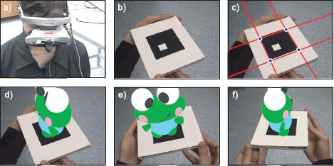
Figure 15.1 Video see-through augmented reality with a planar scene. a) The user views the world through a head mounted display with a camera attached to the front. The images from the camera are analyzed and augmented in near-real time and displayed to the user. b) Here, the world consists of a planar 2D marker. c) The marker corners are found by fitting edges to its sides and finding their intersections. d) The geometric transformation between the 2D positions of the corners on the marker surface and the corresponding positions in the image is computed. This transformation is analyzed to find the rotation and translation of the camera relative to the marker. This allows us to superimpose a 3D object as if it were rigidly attached to the surface of the image. e-f) As the marker is manipulated the superimposed object changes pose appropriately.

where is the 2D observed image position represented as a homogeneous 3-vector and is the 3D point in the world represented as a homogeneous 4-vector. Writing this out explicitly, we have

where the 3D rotation matrix Ω takes a special form with only four unknowns, reflecting the fact that the plane is known to be fronto-parallel.

We can move the distance parameter D into the intrinsic matrix without changing the last of these three equations and equivalently write

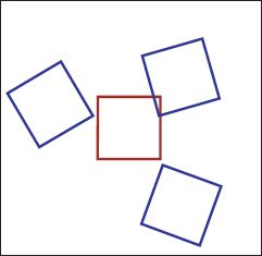
Figure 15.2 The 2D Euclidean transformation describes 2D rigid rotations and translations. The blue squares are all Euclidean transformations of the original red square. The transformation has three parameters: the rotation angle and the translations in the x-and y-directions. When a camera views a fronto-parallel plane at a known distance, the relation between the normalized camera coordinates and the 2D positions on the plane is a Euclidean transformation.

If we now eliminate the effect of this modified intrinsic matrix, by premultiplying both left and right by its inverse we get

where x′ and y′ are camera coordinates that are normalized with respect to this modified intrinsic matrix.

The mapping in Equation 15.4 is known as a Euclidean transformation. It can be equivalently written in Cartesian coordinates as

or for short we may write

where x′ = [x′, y′]^T contains the normalized camera coordinates and w = [u, v]^T is the real-world position on the plane.

The Euclidean transformation describes rigid rotations and translations in the plane (Figure 15.2). Although this transformation appears to take six separate parameters, the rotation matrix Ω can be reexpressed in terms of the rotation angle θ,

and hence the actual number of parameters is three (the two offsets τ_x and τ_y, and the rotation, θ.

15.1.2 Similarity transformation model

Now consider a calibrated camera viewing a fronto-parallel plane at unknown distance D. The relationship between image points x = [x, y]^T and points w = [u, v, 0]^T on the plane is once more given by Equation 15.2. Converting to normalized image coordinates by premultiplying both sides by the inverse of the intrinsic matrix gives

We now multiply each of these three equations by ρ=1/D to get

This is the homogeneous representation of the similarity transformation. However it is usual to incorporate ρ into the constant λ on the left-hand side so that λ← ρλ and into the translation parameters so that τ_x← ρτ_x and τ_y← ρτ_yon the right-hand side to yield

Converting to Cartesian coordinates, we have

or for short,

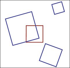
Figure 15.3 The similarity transformation describes rotations, translations, and isotropic scalings. The blue quadrilaterals are all similarity transformations of the original red square. The transformation has four parameters: the rotation angle, the scaling and the translations in the x -and y-directions. When a camera views a fronto-parallel plane at unknown distance, the relation between the normalized camera coordinates and positions on the plane is a similarity.

The similarity transformation is a Euclidean transformation with a scaling (Figure 15.3) and has four parameters: the rotation, the scaling, and two translations.

15.1.3 Affine transformation model

We motivated each of the previous transformations by considering a camera viewing a fronto-parallel plane. Ultimately, we wish to describe the relationship between image points and points on a plane in general position. As an intermediate step, let us generalize the transformations in Equations 15.4 and 15.10 to

where ₁₁, ₁₂, _{21 22} are now unconstrained and can take arbitrary values. This is known as an affine transformation. In Cartesian coordinates, we have

or for short we might write

Note that the camera calibration matrix Λ also has the form of an affine transformation (i.e., a 3 × 3 matrix with two zeros in the bottom row). The product of two affine transformations is a third affine transformation, so if Equation 15.15 is true, then there is also an affine transformation between points on the plane and the original (unnormalized) pixel positions.

The affine transformation encompasses both Euclidean and similarity transformations, but also includes shears (Figure 15.4). However, it is far from general, and a notable restriction is that parallel lines are always mapped to other parallel lines. It has six unknown parameters, each of which can take any value.

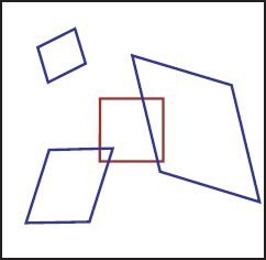
Figure 15.4 The affine transformation describes rotations, translations, scalings, and shears. The blue quadrilaterals are all affine transformations of the original red square. The affine transformation has six parameters: the translations in the x- and y-directions, and four parameters that determine the other effects. Notice that lines that were originally parallel remain parallel after the affine transformation is applied, so in each case the square becomes a parallelogram.

Figure 15.5 Approximating projection of a plane. a) A planar object viewed with a camera with a narrow field of view (long focal length) from a large distance. The depth variation within the object is small compared to the distance from the camera to the plane. Here, perspective distortion is small, and the relationship between points in the image and points on the surface is well approximated by an affine transformation. b) The same planar object viewed with a wide field of view (short focal length) from a short distance. The depth variation within the object is comparable to the average distance from the camera to the plane. An affine transformation cannot describe this situation well. c) However, a projective transformation (homography) captures the relationship between points on the surface and points in this image.

The question remains as to whether the affine transformation really does provide a good mapping between points on a plane and their positions in the image. This is indeed the case when the depth variation of the plane as seen by the camera is small relative to the mean distance from the camera. In practice, this occurs when the viewing angle is not too oblique, the camera is distant, and the field of view is small (Figure 15.5a). In more general situations, the affine transformation is not a good approximation. A simple counterexample is the convergence of parallel train tracks in an image as they become more distant. The affine transformation cannot describe this situation as it can only map parallel lines on the object to parallel lines in the image.

15.1.4 Projective transformation model

Finally, we investigate what really happens when a pinhole camera views a plane from an arbitrary viewpoint. The relationship between a point w = [u, v, 0]^T on the plane and the position x = [x, y]^T to which it is projected is

Combining the two 3 × 3 matrices by multiplying them together, the result is a transformation with the general form

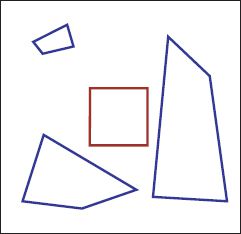
Figure 15.6 The projective transformation (also known as a collinearity or homography) can map any four points in the plane to any other four points. Rotations, translations, scalings, and shears and are all special cases. The blue quadrilaterals are all projective transformations of the original red square. The projective transformation has eight parameters. Lines that were parallel are not constrained to remain parallel after the projective transformation is applied.

and is variously known as a projective transformation, a collinearity, or a homography. In Cartesian coordinates the homography is written as

or for short

The homography can map any four points in the plane to any other four points (Figure 15.6). It is a linear transformation in homogenous coordinates (Equation 15.17) but is nonlinear in Cartesian coordinates (Equation 15.18). It subsumes the Euclidean, similarity, and affine transformations as special cases. It exactly describes the mapping between the 2D coordinates of points on a plane in the real world and their positions in an image of that plane (Figure 15.5c).

Although there are nine entries in the matrix Φ, the homography only contains eight degrees of freedom the entries are redundant with respect to scale. It is easy to see that a constant rescaling of all nine values produces the same transformation, as the scaling factor cancels out of the numerator and denominator in Equation 15.18. The properties of the homography are discussed further in Section 15.5.1.

15.1.5 Adding uncertainty

The four geometric models presented in the preceding sections are deterministic. However, in a real system, the measured positions of features in the image are subject to noise, and we need to incorporate this uncertainty into our models. In particular, we will assume that the positions x_i in the image are corrupted by normally distributed noise with spherical covariance so that, for example, the likelihood for the homography becomes

Figure 15.7 Learning and inference for transformation models. a) Planar object surface (position measured in cm). b) Image (position measured in pixels). In learning, we estimate the parameters of the mapping from points w on the object surface to image positions x_i based on pairs {x_i, w_i}^I_{i = 1} of known correspondences. We can use this mapping to find the position x* in the image to which a point w* on the object surface will project. In inference, we reverse this process: given a position x* in the image, the goal is to establish the corresponding position w* on the object surface.

This is a generative model for the 2D image data x. It can be thought of as a simplified version of the pinhole camera model that is specialized for viewing planar scenes it is a recipe that tells us how to find the position in the image x corresponding to a point w on the surface of the planar object in the world.

The learning and inference problems in this model (Figure 15.7) are

• Learning: we are given pairs of points {x_i, w_i}^I_i=1 where x_i is a position in the image and w_i is the corresponding position on the plane in the world. The goal is to use these to establish the parameters θ of the transformation. For example, in the case of the homography, the parameters θ would comprise the nine entries of the matrix Φ.

• Inference: we are given a new point in the image x*, and our goal is to find the position on the plane w* that projected to it.

We consider these two problems in the following sections.

15.2 Learning in transformation models

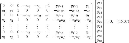
We are given a set of I 2D positions w_i = [u_i, v_i]^T on the surface of the plane and the I corresponding 2D image positions x_i = [x_i, y_i]^T in the image. We select a transformation class of the form trans[w_i, θ]. The goal of the learning algorithm is then to estimate the parameters θ that best map the points w_i to the image positions x_i.

Adopting the maximum likelihood approach, we have

where, as usual, we have taken the logarithm which is a monotonic transformation and hence does not affect the position of the maximum. Substituting in the expression for the normal distribution and simplifying, we get the least squares problem

The solutions to this least squares problem for each of the four transformation types are presented in Sections 15.2.1-15.2.4. The details differ in each case, but they have the common approach of reducing the problem into a standard form for which the solution is known. The algorithms are somewhat involved, and these sections can be skipped on first reading.

15.2.1 Learning Euclidean parameters

The Euclidean transformation is determined by a 2 × 2 rotation matrix Ω and a 2 × 1 translation vector τ = [τ_x, τ_y]^T (Equations 15.4 and 15.5). Each pair of matching points {x_i, w_i} contributes two constraints to the solution (deriving from the x- and y-coordinates). Since there are three underlying degrees of freedom, we will require at least I = 2 pairs of points to get a unique estimate.

Our goal is to solve the problem

with the constraint that Ω is a rotation matrix so that Ω Ω^T = I and |Ω| = 1.

An expression for the translation vector can be found by taking the derivative of the objective function with respect to τ, setting the result to zero and simplifying. The result is the mean difference vector between the two sets of points after the rotation has been applied

where μ_x is the mean of the points {x_i} and μ_w is the mean of the points {w_i}. Substituting this result into the original criterion, we get

Defining matrices B = [x₁ - μ_x, x₂ - μ_x,…, x_I - μ_x] and A = [w₁ - μ_w, w₂ - μ_w,…, w_I - μ_w], we can rewrite the objective function for the best rotation Ω as

where |•|_F denotes the Frobenius norm. This is an example of an orthogonal Procrustes problem. A closed form solution can be found by computing the SVD ULV^T = BA^T, and then choosing = VU^T (see Appendix C.7.3).

15.2.2 Learning similarity parameters

The similarity transformation is determined by a 2 × 2 rotation matrix Ω, a 2 × 1 translation vector τ, and a scaling factor ρ (Equations 15.10 and 15.11). There are four underlying degrees of freedom, so we will require at least I = 2 pairs of matching points {x_i, w_i} to guarantee a unique solution.

The objective function for maximum likelihood fitting of the parameters is

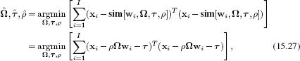
with the constraint that Ω is a rotation matrix so that ΩΩ^T = I and |Ω| = 1.

To optimize this criterion, we compute Ω exactly as for the Euclidean transformation. The maximum likelihood solution for the scaling factor is given by

and the translation can be found using

15.2.3 Learning affine parameters

The affine transformation is parameterized by an unconstrained 2 × 2 matrix Φ and a 2 × 1 translation vector τ (Equations 15.13 and 15.14). There are six unknowns, and so we need a minimum of I = 3 pairs of matching points {x_i, w_i} to guarantee a unique solution. The learning problem can be stated as

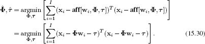
To solve this problem, observe that we can reexpress Φw_i + τ as a linear function of the unknown elements of Φ and τ

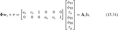
where A_i is a 2 × 6 matrix based on the point w_i, and b contains the unknown parameters. The problem can now be written as

which is a linear least squares problem and can be solved easily (Appendix C.7.1).

15.2.4 Learning projective parameters

The projective transformation or homography is parameterized by a 3 × 3 matrix Φ (Equations 15.17 and 15.18), which is ambiguous up to scale, giving a total of eight degrees of freedom. Consequently, we need a minimum of I = 4 pairs of corresponding points for a unique solution. This neatly matches our expectations: a homography can map any four points in the plane to any other four points, and so it is reasonable that we should need at least four pairs of points to determine it.

The learning problem can be stated as

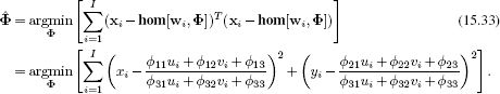
Unfortunately, there is no closed form solution to this nonlinear problem and to find the answer we must rely on gradient-based optimization techniques. Since there is a scale ambiguity, this optimization would normally be carried out under the constraint that the sum of the squares of the elements of Φ is one.

A successful optimization procedure depends on a good initial starting point, and for this we use the direct linear transformation or DLT algorithm. The DLT algorithm uses homogeneous coordinates where the homography is a linear transformation and finds a closed form solution for the algebraic error. This is not the same as optimizing the true objective function (Equation 15.33), but provides a result that is usually very close to the true answer and can be used as a starting point for the nonlinear optimization of the true criterion. In homogeneous coordinates we have

Each homogeneous coordinate can be considered as a direction in 3D space (Figure 14.11). So, this equation states that the left-hand side _i represents the same direction in space as the right-hand side, Φ_i. If this is the case, their cross product must be zero, so that

Writing this constraint in full gives the relations

This appears to provide three linear constraints on the elements of Φ. However, only two of these three equations are independent, so we discard the third. We now stack the first two constraints from each of the I pairs of points {x_i, w_i} to form the system

which has the form A=0.

We solve this system of equations in a least squares sense with the constraint ^T =1 to prevent the trivial solution =0. This is a standard problem (see Appendix C.7.2). To find the solution, we compute the SVD A = ULV^T and choose Φ to be the last column of V. This is reshaped into a 3 × 3 matrix Φ and used as a starting point for the nonlinear optimization of the true criterion (Equation 15.33).

15.3 Inference in transformation models

We have introduced four transformations (Euclidean, similarity, affine, projective) that relate positions w on a real-world plane to their projected positions x in the image and discussed how to learn their parameters. In each case, the transformation took the form of a generative model Pr(x|w). In this section, we consider how to infer the world position w from the image position x.

For simplicity, we will take a maximum likelihood approach to this problem. For the generic transformation trans[w_i, θ], we seek

It is clear that this will be achieved when the image point and the predicted image point agree exactly so that

We can find the w = [u, v]^T that makes this true by moving to homogeneous coordinates. Each of the four transformations can be written in the form

where the exact expressions are given by Equations 15.4, 15.10, 15.13, and 15.17.

To find the position w = [u, v]^T, we simply premultiply by the inverse of the transformation matrix to yield

and then recover u and v by converting back to Cartesian coordinates.

15.4 Three geometric problems for planes

We have introduced transformation models that mapped from 2D coordinates on the plane to 2D coordinates in the image, the most general of which was the homography. Now we relate this model back to the full pinhole camera and revisit the three geometric problems from Chapter 14 for the special case of a planar scene. We will show how to

• learn the extrinsic parameters (compute the geometric relationship between the plane and the camera),

• learn the intrinsic parameters (calibrate from a plane), and

• infer the 3D coordinates of a point in the plane relative to the camera, given its image position.

These three problems are illustrated in Figures 15.8, 15.9, and 15.11, respectively.

15.4.1 Problem 1: learning extrinsic parameters

Given I 3D points {w_i}^I_i=1 that lie on a plane so that w_i = 0, their corresponding projections in the image {x_i}^I_i=1 and known intrinsic matrix Λ, estimate the extrinsic parameters

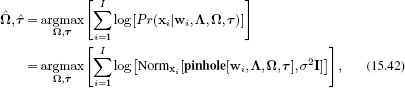
where Ω is a 3 × 3 rotation matrix and τ is a 3 × 1 translation vector (Figure 15.8). The extrinsic parameters transform points w = [u, v, 0] on the plane into the coordinate system of the camera. Unfortunately, this problem (still) cannot be solved in closed form and requires nonlinear optimization. As usual, it is possible to get a good initial estimate for the parameters using a closed form algebraic solution based on homogeneous coordinates.

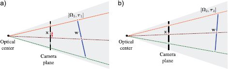
Figure 15.8 Problem 1 - Learning extrinsic parameters. Given points {w_i}^I_i=1 on a plane, their positions {x}^I_i=1 in the image and intrinsic parameters Λ, find the rotation Ω and translation τ relating the camera and the plane. a) When the rotation and translation are wrong, the image points predicted by the model (where the rays strike the image plane) do not agree well with the observed points x. b) When the rotation and translation are correct, they agree well and the likelihood Pr(x|w, Λ, Ω, τ) will be high.

From Equation 15.16, the relation between a homogeneous point on the plane and its projection in the image is

Our approach is to (i) calculate the homography Φ between the points w = [u, v]^T on the plane and the points x = [x, y]^T in the image using the method of Section 15.2.4 and then (ii) decompose this homography to recover the rotation matrix Ω and translation vector τ.

As a first step toward this decomposition, we eliminate the effect of the intrinsic parameters by premultiplying the estimated homography by the inverse of the intrinsic matrix Λ. This gives a new homography Φ′ = Λ⁻¹Φ such that

To estimate the first two columns of the rotation matrix Ω, we compute the SVD of the first two columns of Φ′

and then set

These operations find the closest valid first two columns of a rotation matrix to the first two columns of Φ′ in a least squares sense. This approach is very closely related to the solution to the orthogonal Procrustes problem (Appendix C.7.3).

We then compute the last column [ω₁₃, ω₂₃, ω₃₃]^T of the rotation matrix by taking the cross product of the first two columns: this guarantees a vector that is also length one and is perpendicular to the first two columns, but the sign may still be wrong: we test the determinant of the resulting rotation matrix Ω, and if it is -1, we multiply the last column by -1.

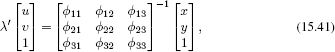
We can now estimate the scaling factor λ′ by taking the average of the scaling factors between these six elements

and this allows us to estimate the translation vector as τ = [′₁₃, ′₂₃, ′₃₃]^T/λ′. The result of this algorithm is a very good initial estimate of the extrinsic matrix [Ω, τ], which can be improved by optimizing the correct objective function (Equation 15.42).

15.4.2 Problem 2: learning intrinsic parameters

In this section, we revisit the problem of learning the intrinsic parameters of the camera (Figure 15.9). This is referred to as camera calibration. In Section 14.5, we developed a method based on viewing a special 3D calibration target. In practice, it is hard to manufacture a three-dimensional object with easy-to-find visual features at precisely known locations. However, it is easy to manufacture a 2D object of this kind. For example, it is possible to print out a checkerboard pattern and attach this to a flat surface (Figure 15.10). Unfortunately, a single view of a 2D calibration object is not sufficient to uniquely identify the intrinsic parameters. However, observing the same pattern from several different viewpoints does suffice.

Hence, the calibration problem can be reformulated as follows: given a planar object, with I distinct 3D points {w_i}^I_i=1 on the surface and the corresponding projections in J images {x_ij}^I,J_{i=1, j=1}, establish the intrinsic parameters in the form of the intrinsic

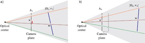
Figure 15.9 Problem 2 - Learning intrinsic parameters. Given a set of points {w_i}^I_i=1 on a plane in the world (blue line) and the 2D positions {x_i}^I_i=1 of these points in an image, find the intrinsic parameters Λ. To do this, we must also simultaneously estimate the extrinsic parameters Ω, τ. a) When the intrinsic and extrinsic parameters are wrong, the prediction of the pinhole camera (where rays strike the image plane) deviates significantly from the known 2D points. b) When they are correct, the prediction of the model will agree with the observed image. To make the solution unique, the plane must be seen from several different angles.

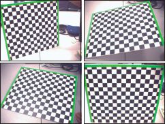
Figure 15.10 Calibration from a plane. It is considerably easier to make a 2D calibration target than to machine an accurate 3D object. Consequently, calibration is usually based on viewing planes such as this checkerboard. Unfortunately, a single view of a plane is not sufficient to uniquely determine the intrinsic parameters. Therefore cameras are usually calibrated using several images of the same plane, where the plane has a different pose relative to the camera in each image.

matrix Λ:

A simple approach to this problem is to use a coordinate ascent technique in which we alternately

• Estimate the J extrinsic matrices relating the object frame of reference to the camera frame of reference in each of the J images,

using the method of the previous section and then,

• Estimate the intrinsic parameters using a minor variation of the method described in Section 14.5:

As for the original calibration method (Section 14.5), a few iterations of this procedure will yield a useful initial estimate of the intrinsic parameters and these can be improved by directly optimizing the true objective function (Equation 15.48). It should be noted that this method is quite inefficient and is described for pedagogical reasons; it is easy both to understand and to implement. A modern implementation would use a more sophisticated technique to find the intrinsic parameters (see Hartley and Zisserman (2004).

15.4.3 Problem 3: inferring 3D position relative to camera

Given a calibrated camera (i.e., camera with known Λ) that is known to be related to a planar scene by extrinsic parameters Ω, τ, find the 3D point w that is responsible for a given 2D position x in the image.

When the scene is planar there is normally a one-to-one relationship between points in the 3D world and points in the image. To compute the 3D point corresponding to a point x, we initiallty infer the position w = [u, v, 0]^T on the plane. We exploit our knowledge of the intrinsic and extrinsic parameters to compute the homography Φ mapping from points in the world to points in the image,

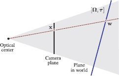
Figure 15.11 Inferring a 3D position relative to the camera. When the object is planar (blue line), there is a one-to-one mapping between points x in the image and points w on the plane. If we know the intrinsic matrix, and the rotation and translation of the plane relative to the camera, we can infer the 3D position w from the observed 2D image point x.

We then infer the coordinates w = [u, v, 0]^T on the plane by inverting this transformation

Finally, we transfer the coordinates back to the frame of reference of the camera to give

15.5 Transformations between images

So far, we have considered transformations between a plane in the world and its image in the camera. We now consider two cameras viewing the same planar scene. The one-to-one mapping from positions on the plane to the positions in the first camera can be described by a homography. Similarly, the one-to-one mapping from positions on the plane to the positions in the second camera can be described by a second homography. It follows that there is a one-to-one mapping from the position in the first camera to the position in the second camera. This can also be described by a homography. The same logic follows for the other transformation types. Consequently, it is very common to find pairs of real-world images that are geometrically related by one of these transformations. For example, the image of the photograph in Figure 15.5a is related by a homography to that in 15.5b.

Let us denote the 3 × 3 matrix mapping points on the plane to points in the first image by T₁. Similarly, we denote the 3 × 3 matrix mapping points on the plane to points in the second image by T₂. To map from image 1 to image 2, we first apply the transformation from image 1 to the plane itself. By the argument of the previous section, this is T₁^-1. Then we apply the transformation from the plane to image 2, which is T₂. The mapping T₃ from image 1 to image 2 is the concatenation of these operations and is hence (Figure 15.12).

15.5.1 Geometric properties of the homography

We’ve seen that transformations between planes in the world and the image plane are described by homographies, and so are transformations between multiple images of a real-world plane. There is another important family of images where the images are related to one another by the homography. Recall that the homography mapping point x₁ to point x₂ is linear in homogeneous coordinates:

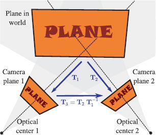
Figure 15.12 Transformations between images. Two cameras view the same planar scene. The relations between the 2D points on this plane and the two images are captured by the 3 × 3 transformation matrices T₁ and T₂, respectively. It follows that the transformation from the first image to the points on the plane is given by T^-1. We can compute the transformation T₃ from the first image to the second image by transforming from the first image to the plane and then transforming from the plane to the second image, giving the final result .

The homogeneous coordinates represent 2D points as directions or rays in a 3D space (Figure 14.11). When we apply a homography to a set of 2D points, we can think of this as applying a linear transformation (rotation, scaling, and shearing) to a bundle of rays in 3D. The positions where the transformed rays strike the plane at w = 1 determine the final 2D positions.

We could yield the same results by keeping the rays fixed and applying the inverse transformation to the plane so that it cuts the rays in a different way. Since any plane can be mapped to any other plane by a linear transformation, it follows that the images created by cutting a ray bundle with different planes are all related to one another by homographies (Figure 15.13). In other words, the images seen by different cameras with the pinhole in the same place are related by homographies. So, for example, if a camera zooms (the focal length increases), then the images before and after the zoom are related by a homography.

This relationship encompasses an important special case (Figure 15.14). If the camera rotates but does not translate, then the image plane still intersects the same set of rays. It follows that the projected points x₁ before the rotation and the projected points x₂ after the rotation are related by a homography. It can be shown that the homography Φ mapping from image 1 to image 2 is given by

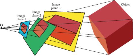
Figure 15.13 Geometric interpretation of homography. A ray bundle is formed by connecting rays from an optical center to points on a real-world object (the cube). A set of planes cut the ray bundle, forming a series of images of the cube. Each of these images is related to every other by a homography.

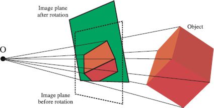
Figure 15.14 Images under pure camera rotation. When the camera rotates but does not translate, the bundle of rays remains the same, but is cut by a different plane. It follows that the two images are related by a homography.

where Λ is the intrinsic matrix and Ω₂ is the rotation matrix that maps the coordinate system of the second camera to the first. This relationship is exploited when we stitch together images to form panoramas (Section 15.7.2).

In conclusion, the homography maps between

• Points on a plane in the world and their positions in an image,

• Points in two different images of the same plane, and

• Two images of a 3D object where the camera has rotated but not translated.

15.5.2 Computing transformations between images

In the previous sections we have argued that it is common for two images to be related to one another by a homography. If we denote the points in image 1 by x_i and their corresponding positions in image 2 as y_i, then we could for example describe the mapping as a homography

This method ascribes all of the noise to the first image and it should be noted that it is not quite correct: we should really build a model that explains both sets of image data with a set of hidden variables representing the original 3D points so that the estimated point positions in each image are subject to noise. Nonetheless, the model in Equation 15.56 works well in practice. It is possible to learn the parameters using the technique of Section 15.2.

15.6 Robust learning of transformations

We have discussed transformation models that can be used either to (i) map the positions of points on a real-world plane to their projections in the image or (ii) map the positions of points in one image to their corresponding positions in another. Until now, we have assumed that we know a set of corresponding points from which to learn the parameters of the transformation model. However, establishing these correspondences automatically is a challenging task in itself.

Let us consider the case where we wish to compute a transformation between two images. A simple method to establish correspondences would be to compute interest points in each image and to characterize the region around each point using a region descriptor such as the SIFT descriptor (Section 13.3.2). We could then greedily associate points based on the similarity of the region descriptors (as in Figure 15.17c-d). Depending on the scene, this is likely to produce a set of matches that are 70-90% correct. Unfortunately the remaining erroneous correspondences (which we will call outliers) can severely hamper our ability to compute the transformation between the images. To cope with this problem, we need robust learning methods.

15.6.1 RANSAC

Random sample consensus or RANSAC is a general method for fitting models to data where the data are corrupted by outliers. These outliers violate the assumptions of the underlying probability model (usually a normal distribution) and can cause the estimated parameters to deviate significantly from their correct values.

For pedagogical reasons, we will describe RANSAC using the example of linear regression. We will subsequently return to the problem of learning parameters in transformation models. The linear regression model is

and was discussed at length in Section 8.1. Figure 15.15 shows an example of the predicted mean for y when we fit the model to data with two outliers. The fit has been unduly influenced by the outliers and no longer describes the data well.

The goal of RANSAC is to identify which points are outliers and to eliminate them from the final fit. This is a chicken and egg problem: if we had the final fit, then it would be easy to identify the outliers (they are not well described by the model), and if we knew which points were outliers, it would be easy to compute the final fit.

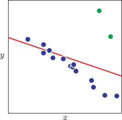
Figure 15.15 Motivation for random sample consensus (RANSAC). The majority of this data set (blue points) can be explained well by a linear regression model, but there are two outliers (green points). Unfortunately, if we fit the linear regression model to all of this data, the mean prediction (red line) is dragged toward the outliers and no longer describes the majority of the data well. The RANSAC algorithm circumvents this problem by establishing which datapoints are outliers and fitting the model to the remaining data.

RANSAC works by repeatedly fitting models based on random subsets of the data. The hope is that sooner or later, there will be no outliers in the chosen subset, and so we will fit a good model. To enhance the probability of this happening, RANSAC chooses subsets of the minimal size required to uniquely fit the model. For example, in the case of the line, it would choose subsets of size two.

Having chosen a minimal subset of datapoints and fitted the model, RANSAC assesses its quality. It does this by classifying points as inliers or outliers. This requires some knowledge about the expected amount of variation around the true model. For linear regression this means we need some prior knowledge of the variance parameter σ². If a datapoint exceeds the expected variation (perhaps two standard deviations from the mean), then it is classified as an outlier. Otherwise, it is an inlier. For each minimal subset of data, we count the number of inliers.

We repeat this procedure a number of times: on each iteration we choose a random minimal subset of points, fit a model, and count the number of datapoints that agree (the inliers). After a predetermined number of iterations, we then choose the model that had the most inliers and refit the model from these alone.

The complete RANSAC algorithm hence proceeds as follows (Figure 15.16):

1. Randomly choose a minimal subset of data.

2. Use this subset to estimate the parameters.

3. Compute the number of inliers for this model.

4. Repeat steps 1-3 a fixed number of times.

5. Reestimate model using inliers from the best fit.

If we know the degree to which our data are polluted with outliers, it is possible to estimate the number of iterations that provide any given chance of finding the correct answer.

Now let us return to the question of how to apply the model to fitting geometric transformations. We will use the example of a homography (Equation 15.56). Here we repeatedly choose subsets of hypothesized matches between the two images. The size of the subset is chosen to be four as this is the minimum number of pairs of points that are needed to uniquely identify the eight degrees of freedom of the homography.

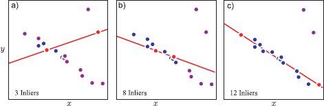
Figure 15.16 RANSAC procedure. a) We select a random minimal subset of points to fit the line (red points). We fit the line to these points and count how many of the other points agree with this solution (blue points). These are termed inliers. Here there are only three inliers. b,c) This procedure is repeated with different minimal subsets of points. After a number of iterations we choose the fit that had the most inliers. We refit the line using only the inliers from this fit.

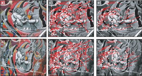
Figure 15.17 Fitting a homography with RANSAC. a,b) Original images of a textured plane. c,d) 162 strongest matches selected by greedy method. In each case the associated line travels from the interest point to the position of its match in the other image. These matches are clearly polluted by outliers. e,f) Model fitted from 102 inliers identified by applying 100 iterations of RANSAC. These matches form a coherent pattern as they are all described by a homography.

For each subset, we count the number of inliers by evaluating Equation 15.56 and selecting those where the likelihood exceeds some predetermined value. In practice, this means measuring the distance between the points x_i in the first image and the mapped position hom[y, Φ] of the points from the second image. After repeating this many times, we identify the trial with the most inliers (Figure 15.17) and recompute the model from these inliers alone.

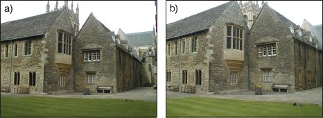
Figure 15.18 Piecewise planarity. a) Although this scene is clearly not well described by a plane, it is well described by a set of planes. b) Consequently, the mapping to this second image of the same scene can be described by a set of homographies. Images from Oxford Colleges dataset.

15.6.2 Sequential RANSAC

Now let us look at a more challenging task. So far, we assumed that one set of points could be mapped to another using a single transformation model. However, many scenes containing man-made objects are piecewise planar (Figure 15.18). It follows that images of such scenes are related by piecewise homographies. In this section, we will consider methods for fitting this type of model.

The first approach is sequential RANSAC. The idea is simple: we fit a single homography to the scene using the RANSAC method. In principle this will correctly fit a model to one of the planes in the image and reject all the other points as outliers. We then remove the points that belong to this plane (i.e., the inliers to the final homography) and repeat the procedure on the remaining points. Ideally, each iteration will identify a new plane in the image.

Unfortunately, this method does not work well in practice (Figure 15.19) for two reasons. First, the algorithm is greedy: any matches that are erroneously incorporated into, or missed by one of the earlier models cannot be correctly assigned later. Second, the model has no notion of spatial coherence, ignoring the intuition that nearby points are more likely to belong to the same plane.

15.6.3 PEaRL

The Propose, Expand and Re-Learn or PEaRL algorithm solves both of these problems. In the “propose” stage, K hypothetical models are generated where K is usually of the order of several thousand. This can be achieved by using a RANSAC type procedure in which minimal subsets of points are chosen, a model is fitted, and the inliers are counted. This is done repeatedly until we have several thousand models {Φ_k}^K_k=1 that each have a reasonable degree of support.

In the “expand” stage, we model the assignment of matched pairs to the proposed models as a multilabel Markov random field. We associate a label l_i ∈ [1, 2,…, K] to each match {x_i, y_i} where the value of the label determines which one of the K models is present at this point. The likelihood of each data pair {x_i, y_i} under the k^th model is given by

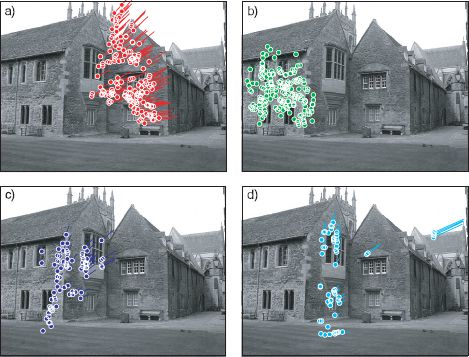
Figure 15.19 Sequential fitting of homographies mapping between images in Figure 15.18 using RANSAC. a) Running the RANSAC fitting procedure once identifies a set of points that all lie on the same plane in the image. b) Running the RANSAC procedure again on the points that were not explained by the first plane identifies a second set of points that lie on a different plane. c) Third iteration. The plane discovered does not correspond to a real plane in the scene. d) Fourth iteration. The model erroneously associates parts of the image which are quite separate. This sequential approach fails for two reasons. First, it is greedy and cannot recover from earlier errors. Second, it does not encourage spatial smoothness (nearby points should belong to the same model).

To incorporate spatial coherence, we choose a prior over the labels that encourages neighbors to take similar values. In particular, we choose an MRF with a Potts model potential

where Z is the constant partition function, w_ij is a weight associated with the pair of matches i and j, and δ[•] is a function that returns 1 when the argument is zero and returns 0 otherwise. The neighborhood _i of each point must be chosen in advance. One simple technique is to compute the K-nearest neighbors for each point in the first image and declare two points to be neighbors if either is in the other’s set of closest neighbors. The weights w_ij are chosen so that points that are close in the image are more tightly coupled than points that are distant.

The goal of the “expand” stage is then to infer the labels l_i and hence the association between models and datapoints. This can be accomplished using the alpha expansion algorithm (Section 12.4.1). Finally, having associated each datapoint with one of the models, we move to the “re-learn” stage. Here, we reestimate the parameters of each model based on the data that was associated with it. The “expand” and “re-learn” stages are iterated until no further progress is made. At the end of this process, we throw away any models that do not have sufficient support in the final solution (Figure 15.20).

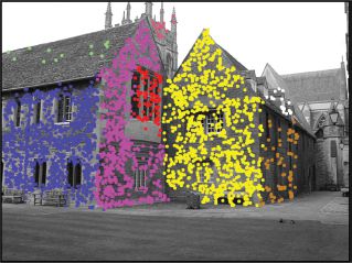
Figure 15.20 Results of the PEaRL algorithm. It formulates the problem as inference in a multilabel MRF. The MRF label associated with each matching pair denotes the index of one of a set of possible models. Inferring these labels is alternated with refining the parameters of the proposed models. The colored points denote different labels in the final solution. The algorithm has successfully identified many of the surfaces in the scene. Adapted from Isack and Boykov (2012). ©2012 Springer.

15.7 Applications

In this section we present two examples of the techniques in this chapter. First, we discuss augmented reality in which we attempt to render an object onto a plane in the scene. This application exploits the fact that there is a homography between the image of the plane and the original object surface and uses the method of Section 15.4.1 to decompose this homography to find the relative position of the camera and the plane. Second, we discuss creating visual panoramas. The method exploits the fact that multiple images taken from a camera that has rotated but not translated are all related by homographies.

15.7.1 Augmented reality tracking

Figure 15.1 shows an example of augmented reality tracking. To accomplish this, the following steps were taken. First, the four corners of the marker are found as in Figure 15.1c; the marker was designed so that the corners can be easily identified using a set of image-processing operations. In brief, the image is thresholded, and then connected dark regions are found. The pixels around the edge of each region are identified. Then four 2D lines are fit to the edge pixels using sequential RANSAC. Regions that are not well explained by four lines are discarded. The only remaining region in this case is the square marker.

The positions where the fitted lines intersect provides four points {x_i}⁴_i=1 in the image, and we know the corresponding positions {w_i}⁴_i=1 in cm that occur on the surface of the planar marker. It is assumed that the camera is calibrated, and so we know the intrinsic matrix Λ. We can now compute the extrinsic parameters Ω, τ using the algorithm from Section 15.4.1.

To render the graphical object, we first set up a viewing frustum (the graphics equivalent of the “camera”) so that it has the same field of view as specified by the intrinsic parameters. Then we render the model from the appropriate perspective using the extrinsic parameters as the modelview matrix. The result is that the object appears to be attached rigidly to the scene.

In this system, the points on the marker were found using a sequence of image-processing operations. However, this method is rather outdated. It is now possible to reliably identify natural features on an object so there is no need to use a marker with any special characteristics. One way to do this is to match SIFT features between a reference image of the object and the current scene. These interest point descriptors are invariant to image scaling and rotation, and for textured objects it is usually possible to generate a high percentage of correct matches. RANSAC is used to eliminate any mismatched pairs.

However, SIFT features are themselves relatively slow to compute. Lepetit et al. (2005) described a system that applies machine learning techniques to identify objects at interactive speeds (Figure 5.21). They first identify K stable keypoints (e.g., Harris corners) on the object to be tracked. They then create a training set for each keypoint by subjecting the region around it to a large number of random affine transformations. Finally, they train a multiclass classification tree that takes a new keypoint and assigns it to match one of the K original points. At each branch of the tree, the decision is made by a pairwise intensity comparison. This system works very quickly and reliably matches most of the feature points. Once more, RANSAC can be used to eliminate any erroneous matches.

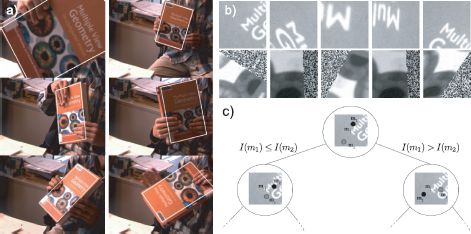
Figure 15.21 Robust tracking using keypoints. a) Lepetit et al. (20005) presented a system that automatically tracked objects such as this book. b) In the learning stage, the regions around the keypoints were subjected to a number of random affine transformations. c) Keypoints in the image were classified as belonging to a known keypoint on the object, using a tree-based classifier that compared the intensity at nearby points. Adapted from Lepetit et al. (2005). ©2005 IEEE.

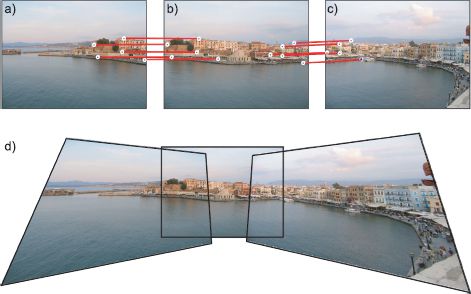
Figure 15.22 Computing visual panoramas. a-c) Three images of the same scene where the camera has rotated but not translated. Five matching points have been identified by hand between each pair. d) A panorama can be created by mapping the first and third images into the frame of reference of the second image.

15.7.2 Visual panoramas

A second application of the ideas of this chapter is the computation of visual panoramas. Recall that a set of pictures that are taken by rotating a camera about the optical center are all related by homographies. Hence, if we take pictures of this kind that are partially overlapping, it is possible to map them all into one large image. This process is known as image mosaicing.

An example is shown in Figure 15.22. This was constructed by placing the second (middle) photo into the center of a much larger empty image. Then 5 matches were identified by hand between this expanded second image and the first image and the homography from the expanded second image to the first image was computed. For each empty pixel in the expanded second image we compute the position in the first image using this homography. If this falls within the image boundaries, we copy the pixel value.

This process can be completely automated by finding features and fitting a homography to each pair of images using a robust technique such as RANSAC. In a real system, the final result is typically projected onto a cylinder and unrolled to give a more visually pleasing result.

Discussion

This chapter has presented a number of important ideas. First, we discussed a family of transformations and how each can be related to a camera viewing the scene under special conditions. These transformations are used widely within machine vision and we will see them exploited in Chapters 17-19. Second, we discussed a more practical method for camera calibration based on viewing a plane at a number of different orientations. Finally, we have also presented RANSAC, which is a robust method to fit models, even in the presence of noisy observations.

Notes

Transformations: For more information concerning the hierarchy of 2D transformations, consult Hartley and Zisserman (2004). The closed form solutions for the rotation and similarity transformations are special cases of Procrustes problems. Many more details about this type of problem can be found in Gower and Dijksterhuis (2004). The direct linear transformation algorithm for estimating the homography dates back to at least Sutherland (1963). Hartley and Zisserman (2004) present a detailed discussion of different objective functions for estimating homographies. In this chapter, we have discussed the estimation of transformations from point matches. However, it is also possible to compute transformations from other geometric primitives. For example, methods exist to compute the homography from matched lines (see Problem 15.3), a combination of points and lines Murino et al. (2002), or conics Sugimoto 2000).

Robust estimation: The RANSAC algorithm is due to Fischler and Bolles (1981). It has spawned many variants, the most notable of which is MLESAC (Torr and Zisserman 2000) which puts this fitting method on a sound probabilistic footing (see Problem 15.13 for a related model). Chum et al. (2005) and present variants of RANSAC that can cope with degenerate data (where the model is nonunique). Torr (1998) and Vincent and Laganiere (2001) used RANSAC to estimate multiple geometric entities sequentially. Both Raguram et al. (2008) and Choi et al. (2009) present recent quantitative comparisons of variations of the RANSAC algorithm. The PEaRL algorithm is due to Isack and Boykov(2012). In the original paper, they also include an extra cost, which encourages parsimony (to describe the data with as few models as possible). Other approaches to robust estimation include (i) the use of long-tailed distributions such as the t-distribution (Section 7.5), (ii) M-estimators (Huber 2009), which replace the least-squares criterion with another function that penalizes large deviations less stringently, and (iii) the self-explanatory least median of squares regression (Rousseeuw 1984).

Augmented reality: Pose estimation for augmented reality initially relied on detecting special patterns in the scene known as fiducial markers. Early examples used circular patterns (e.g. Cho et al. 1998; state et al. 1996), but these were largely supplanted by square markers (e.g., Rekimoto 1998; Kato et al. 2000; Kato and Billinghurst 1999; Koller et al. 1997). The system described in the text is ARToolkit (Kato and Billinghurst 1999; Kato et al. 2000) and can be downloaded from http://www.hitl.washington.edu/artoolkit/.

Other systems have used “natural image features.” For example, Harris (1992) estimated the pose of an object using line segments. Simon et al. (2000) and Simon and Berger (2002) estimated the pose of planes in the image using the results of a corner detector. More information about computing the pose of a plane can be found in Sturm (2000).

More recent systems have used interest point detectors such as SIFT features, which are robust to changes in illumination and pose (e.g., Skrypnyk and Lowe 2004). To increase the speed of systems, features are matched using machine learning techniques (Lepetit and Fua 2006; Özuysal et al. 2010), and current systems can now operate at interactive speeds on mobile hardware (Wagner et al. 2008). A review of methods to estimate and track the pose of rigid objects can be found in Lepetit and Fua (2005).

Calibration from a plane: Algorithms for calibration from several views of a plane can be found in Sturm and Maybank (1999) and Zhang (2000). They are now used much more frequently than calibration based on 3D objects, for the simple reason that accurate 3D objects are harder to manufacture.

Image mosaics: The presented method for computing a panorama by creating a mosaic of images is naïve in a number of ways. First, it is more sensible to explicitly estimate the rotation matrix and calibration parameters rather than the homography (Szeliski and Shum 1997; Shum and Szeliski 2000; Brown and Lowe 2007). Second, the method that we describe projects all of the images onto a single plane, but this does not work well when the panorama is too wide as the images become increasingly distorted. A more sensible approach is to project images onto a cylinder (Szeliski 1996; Chen 1995) which is then unrolled and displayed as an image. Third, the method to blend together images is not discussed. This is particularly important if there are moving objects in the image. A good review of these and other issues can be found in Szeliski (2006) and Chapter 9 of Szeliski (2010).

Problems

15.1 The 2D point x₂ is created by a rotating point x₁ using the rotation matrix Ω₁ and then translating it by the translation vector τ₁ so that

Find the parameters Ω₂ and τ₂ of the inverse transformation

in terms of the original parameters Ω₁ and τ₁.

15.2 A 2D line can be as expressed as ax + by + c =0 or in homogeneous terms

where l = [a, b, c]. If points are transformed so that

what is the equation of the transformed line?

15.3 Using your solution from Problem 15.2, develop a linear algorithm for estimating a homography based on a number of matched lines between the two images (i.e., the analogue of the DLT algorithm for matched lines).

15.4 A conic (see Problem 14.6) is defined by

where C is a 3 × 3 matrix. If the points in the image undergo the transformation

then what is the equation of the transformed conic?

15.5 All of the 2D transformations in this chapter (Euclidean, similarity, affine, projective) have 3D equivalents. For each class write out the 4 × 4 matrix that describes the 3D transformation in homogeneous coordinates. How many independent parameters does each model have?

15.6 Devise an algorithm to estimate a 3D affine transformation based on two sets of matching 3D points. What is the minimum number of points required to get a unique estimate of the parameters of this model?

15.7 A 1D affine transformation acts on 1D points x as x′ = ax + b. Show that the ratio of two distances is invariant to a 1D affine transformation so that

15.8 A 1D projective transformation acts on 1D points x as x′ = (ax + b)/(cx + d). Show that the cross-ratio of distances is invariant to a 1D projective transformation so that

It was proposed at one point to exploit this type of invariance to recognize planar objects under different transformations (Rothwell et al. 1995). However, this is rather impractical as it assumes that we can identify a number of the points on the object in a first place.

15.9 Show that Equation 15.36 follows from Equation 15.35.

15.10 A camera with intrinsic matrix λ and extrinsic parameters Ω = I, τ = 0 takes an image and then rotates to a new position Ω = Ω₁, τ = 0 and takes a second image. Show that the homography relating these two images is given by

15.11 Consider two images of the same scene taken from a camera that rotates, but does not translate between taking the images. What is the minimum number of point matches required to recover a 3D rotation between two images taken using a camera where the intrinsic matrix is known?

15.12 Consider the problem of computing a homography from point matches that include outliers. If 50 percent of the initial matches are correct, how many iterations of the RANSAC algorithm would we expect to have to run in order to have a 95 percent chance of computing the correct homography?

15.13 A different approach to fitting transformations in the presence of outliers is to model the uncertainty as a mixture of two Gaussians. The first Gaussian models the image noise, and the second Gaussian, which has a very large variance, accounts for the outliers. For example, for the affine transformation we would have

where λ is the probability of being an inlier, σ² is the image noise, and σ₀² is the large variance that accounts for the outliers. Sketch an approach to learning the parameters σ², Φ, τ, and λ of this model. You may assume that σ₀² is fixed. Identify a possible weakness of this model.

15.14 In the description of how to compute the panorama (Section 15.7.2), it is suggested that we take each pixel in the central image and transform it into the other images and then copy the color. What is wrong with the alternate strategy of taking each pixel from the other images and transforming them into the central image?