Computer Vision: Models, Learning, and Inference (2012)
Part V
Models for geometry
Chapter 16
Multiple cameras
This chapter extends the discussion of the pinhole camera model. In Chapter 14 we showed how to find the 3D position of a point based on its projections into multiple cameras. However, this approach was contingent on knowing the intrinsic and extrinsic parameters of these cameras, and this information is often unknown. In this chapter we discuss methods for reconstruction in the absence of such information. Before reading this chapter, readers should ensure that they are familiar with the mathematical formulation of the pinhole camera (Section 14.1).
To motivate these methods, consider a single camera moving around a static object. The goal is to build a 3D model from the images taken by the camera. To do this, we will also need to simultaneously establish the properties of the camera and its position in each frame. This problem is widely known as structure from motion, although this is something of a misnomer as both “structure” and “motion” are recovered simultaneously.
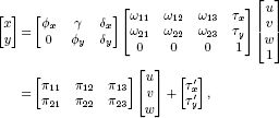
The structure from motion problem can be stated formally as follows. We are given J images of a rigid object that is characterized by I distinct 3D points {wi}i=1I. The images are taken with the same camera at a series of unknown positions. Given the projections {xij}I,Ji=1, j=1 of the I points in the J images, establish the 3D positions {wi}Ii=1 of the points in the world, the fixed intrinsic parameters Λ, and the extrinsic parameters {Ωj, τj}j=1J for each image
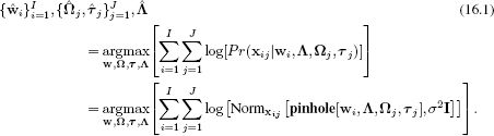
Since this objective function is a based on the normal distribution we can reformulate it as a least squares problem of the form
in which the goal is to minimize the total squared distance between the observed image points and those predicted by the model. This is known as the squared reprojection error. Unfortunately, there is no simple closed form solution for this problem, and we must ultimately rely on nonlinear optimization. However, to ensure that the optimization converges, we need good initial estimates of the unknown parameters.
To simplify our discussion, we will concentrate first on the case where we have J = 2 views, and the intrinsic matrix Λ is known. We already saw how to estimate 3D points given known camera positions in Section 14.6, so the unresolved problem is to get good initial estimates of the extrinsic parameters. Surprisingly, it is possible to do this based on just examining the positions of corresponding points without having to reconstruct their 3D world positions. To understand why, we must first learn more about the geometry of two views.
16.1 Two-view geometry
In this section, we show that there is a geometric relationship between corresponding points in two images of the same scene. This relationship depends only on the intrinsic parameters of the two cameras and their relative translation and rotation.
16.1.1 The epipolar constraint
Consider a single camera viewing a 3D point w in the world. We know that w must lie somewhere on the ray that passes through the optical center and position x1 on the image plane (Figure 16.1). However, from one camera alone, we cannot know how far along this ray the point is.
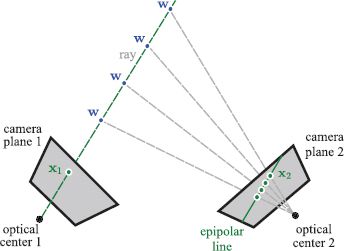
Figure 16.1 Epipolar line. Consider point x1 in the first image. The 3D point w that projected to x1 must lie somewhere along the ray that passes from the optical center of camera 1 through the position x1 in the image plane (dashed green line). However, we don’t know where along that ray it lies (4 possibilities shown). It follows that x2, the projected position in camera 2, must lie somewhere on the projection of this ray. The projection of this ray is a line in image 2 and is referred to as an epipolar line.
Now consider a second camera viewing the same 3D world point. We know from the first camera that this point must lie along a particular ray in 3D space. It follows that the projected position x2 of this point in the second image must lie somewhere along the projection of this ray in the second image. The ray in 3D projects to a 2D line which is known as an epipolar line.
This geometric relationship tells us something important: for any point in the first image, the corresponding point in the second image is constrained to lie on a line. This is known as the epipolar constraint. The particular line that it is constrained to lie on depends on the intrinsic parameters of the cameras and the extrinsic parameters (i.e., the relative translation and rotation of the two cameras).
The epipolar constraint has two important practical implications.
1. Given the intrinsic and extrinsic parameters, we can find point correspondences relatively easily: for a given point in the first image, we only need to perform a 1D search along the epipolar line in the second image for the corresponding position.
2. The constraint on corresponding points is a function of the intrinsic and extrinsic parameters; given the intrinsic parameters, we can use the observed pattern of point correspondences to determine the extrinsic parameters and hence establish the geometric relationship between the two cameras.
16.1.2 Epipoles
Now consider a number of points in the first image. Each is associated with a ray in 3D space. Each ray projects to form an epipolar line in the second image. Since all the rays converge at the optical center of the first camera, the epipolar lines must converge at a single point in the second image plane; this is the image in the second camera of the optical center of the first camera and is known as the epipole (Figure 16.2). Similarly, points in image 2 induce epipolar lines in image 1, and these epipolar lines converge at the epipole in image 1. This is the image in camera 1 of the optical center of camera 2.
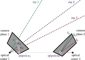
Figure 16.2 Epipoles. Consider several observed points {xi}Ii=1 in image 1. For each point, the corresponding 3D world position wi lies on a different ray. Each ray projects to an epipolar line li in image 2. Since the rays converge in 3D space at the optical center of camera 1, the epipolar lines must also converge. The point where they converge is known as the epipole e2. It is the projection of the optical center of camera 1 into camera 2. Similarly, the epipole e1 is the projection of the optical center of camera 2 into camera 1.
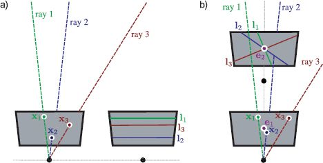
Figure 16.3 Epipolar lines and epipoles. a) When the camera movement is a pure translation perpendicular to the optical axis (parallel to the image plane), the epipolar lines are parallel and the epipole is at infinity. b) When the camera movement is a pure translation along the optical axis, the epipoles are in the center of the image and the epipolar lines form a radial pattern.
The epipoles are not necessarily within the observed images: the epipolar lines may converge to a point outside the visible area. Two common cases are illustrated in Figure 16.3. When the cameras are oriented in the same direction (i.e., no relative rotation) and the displacement is perpendicular to their optical axes (Figure 16.3a), then the epipolar lines are parallel and the epipoles (where they converge) are hence at infinity. When the cameras are oriented in the same direction and the displacement is parallel to their optical axes (Figure 16.3b), then the epipoles are in the middle of the images, and the epipolar lines form a radial pattern. These examples illustrate that the pattern of epipolar lines provides information about the relative position and orientation of the cameras.
16.2 The essential matrix
Now we will capture these geometric intuitions in the form of a mathematical model. For simplicity, we will assume that the world coordinate system is centered on the first camera so that the extrinsic parameters (rotation and translation) of the first camera are {I, 0}. The second camera may be in any general position {Ω, τ}. We will further assume that the cameras are normalized so that Λ1 = Λ2 = I. In homogeneous coordinates, a 3D point w is projected into the two cameras as
![]()
where ![]() 1 is the observed position in the first camera,
1 is the observed position in the first camera, ![]() 2 is the observed position in the second camera, and both are expressed in homogeneous coordinates.
2 is the observed position in the second camera, and both are expressed in homogeneous coordinates.
Expanding the first of these relations, we get
This simplifies to
![]()
By a similar process, the projection in the second camera can be written as
![]()
Finally, substituting Equation 16.5 into Equation 16.6 yields
![]()
This relationship represents a constraint between the possible positions of corresponding points x1 and x2 in the two images. The constraint is parameterized by the rotation and translation {Ω, τ} of the second camera relative to the first.
We will now manipulate the relationship in Equation 16.7 into a form that can be more easily related to the epipolar lines and the epipoles. We first take the cross product of both sides with the translation vector τ. This removes the last term as the cross product of any vector with itself is zero. Now we have
![]()
Then we take the inner product of both sides with ![]() 2. The left-hand side disappears since τ ×
2. The left-hand side disappears since τ × ![]() 2 must be perpendicular to
2 must be perpendicular to ![]() 2, and so we have
2, and so we have
![]()
where we have also divided by the scaling factors λ1 and λ2. Finally, we note that the cross product operation τ × can be expressed as multiplication by the rank 2 skew-symmetric 3 × 3 matrix τ × :
![]()
Hence Equation 16.9 has the form
![]()
where E = τ × Ω is known as the essential matrix. Equation 16.11 is an elegant formulation of the mathematical constraint between the positions of corresponding points x1 and x2 in two normalized cameras.
16.2.1 Properties of the essential matrix
The 3 × 3 essential matrix captures the geometric relationship between the two cameras and has rank 2 so that [E] = 0. The first two singular values of the essential matrix are always identical, and the third is zero. It depends only on the rotation and translation between the cameras, each of which has three parameters, and so one might think it would have 6 degrees of freedom. However, it operates on homogeneous variables ![]() 1 and
1 and ![]() 2 and is hence ambiguous up to scale: multiplying all of the entries of the essential matrix by any constant does not change its properties. For this reason, it is usually considered as having 5 degrees of freedom.
2 and is hence ambiguous up to scale: multiplying all of the entries of the essential matrix by any constant does not change its properties. For this reason, it is usually considered as having 5 degrees of freedom.
Since there are fewer degrees of freedom than there are unknowns, the nine entries of the matrix must obey a set of algebraic constraints. These can be expressed compactly as
![]()
These constraints are sometimes exploited in the computation of the essential matrix, although in this volume we use a simpler method (Section 16.4).
The epipolar lines are easily retrieved from the essential matrix. The condition for a point being on a line is ax + by +c = 0 or
![]()
In homogeneous co-ordinates, this can be written as l![]() = 0 where l = [a, b, c] is a 1 × 3 vector representing the line.
= 0 where l = [a, b, c] is a 1 × 3 vector representing the line.
Now consider the essential matrix relation
![]()
Since ![]() 2TE is a 1 × 3 vector, this relationship has the form l1
2TE is a 1 × 3 vector, this relationship has the form l1![]() 1 = 0. The line l1 =
1 = 0. The line l1 = ![]() 2TE is the epipolar line in image 1 due to the point x2 in image 2. By a similar argument, we can find the epipolar line l2 in the second camera due to the point x1 in the first camera. The final relations are
2TE is the epipolar line in image 1 due to the point x2 in image 2. By a similar argument, we can find the epipolar line l2 in the second camera due to the point x1 in the first camera. The final relations are
![]()
The epipoles can also be extracted from the essential matrix. Every epipolar line in image 1 passes through the epipole ![]() ;1, so at the epipole
;1, so at the epipole ![]() ;1 we have
;1 we have ![]() 2TE
2TE![]() ;1 = 0 for all
;1 = 0 for all ![]() 2. This implies that
2. This implies that ![]() ;1 must lie in the right null-space of E (see Appendix C.2.7). By a similar argument, the epipole
;1 must lie in the right null-space of E (see Appendix C.2.7). By a similar argument, the epipole ![]() ;2 in the second image must lie in the left null space of E. Hence, we have the relations
;2 in the second image must lie in the left null space of E. Hence, we have the relations
![]()
In practice, the epipoles can be retrieved by computing the singular value decomposition E = ULVT of the essential matrix and setting ![]() ;1 to the last column of V and
;1 to the last column of V and ![]() ;2 to the last row of U.
;2 to the last row of U.
16.2.2 Decomposition of essential matrix
We saw previously that the essential matrix is defined as
![]()
where Ω and τ are the rotation matrix and translation vector that map points in the coordinate system of camera 2 to the coordinate system of camera 1, and τ× is a 3 × 3 matrix derived from the translation vector.
We will defer the question of how to compute the essential matrix from a set of corresponding points until Section 16.3. For now, we will concentrate on how to decompose a given essential matrix E to recover this rotation Ω and translation τ. This is known as the relative orientation problem.
In due course, we shall see that whereas we can compute the rotation exactly, it is only possible to compute the translation up to an unknown scaling factor. This remaining uncertainty reflects the geometric ambiguity of the system; from the images alone, we cannot tell if these cameras are far apart and looking at a large distant object or close together and looking at a small nearby object.
To decompose E, we define the matrix
![]()
and then take the singular value decomposition E = ULVT. We now choose
![]()
It is convention to set the magnitude of the translation vector τ that is recovered from the matrix τ × to unity.
The preceding decomposition is not obvious, but it is easily checked that multplying the derived expressions for τ × and Ω yields E = ULVT. This method assumes that we started with a valid essential matrix where the first two singular values are identical and the third is zero. If this is not the case (due to noise), then we can substitute L′ = diag[1, 1, 0] for L in the solution for τ×. For a detailed proof of this decomposition, consult Hartley and Zisserman(2004).
This solution is only one of four possible combinations of Ω and τ that are compatible with E (Figure 16.4). This fourfold ambiguity is due to the fact that the pinhole model cannot distinguish between objects that are behind the camera (and are not imaged in real cameras) and those that are in front of the camera.
Part of the uncertainty is captured mathematically by our lack of knowledge of the sign of the essential matrix (recall it is ambiguous up to scale) and hence the sign of the recovered translation. Hence, we can generate a second solution by multiplying the translation vector by -1. The other component of the uncertainty results from an ambiguity in the decomposition of the essential matrix; we can equivalently replace W for W-1 in the decomposition procedure, and this leads to two more solutions.
Fortunately, we can resolve this ambiguity using a corresponding pair of points from the two images. For each putative solution, we reconstruct the 3D position associated with this pair (Section 14.6). For one of the four possible combinations of Ω, τ, the point will be in front of both cameras, and this is the correct solution. In each of the other three cases, the point will be reconstructed behind one or both of the cameras (Figure 16.4). For a robust estimate, we would repeat this procedure with a number of corresponding points and base our decision on the total number of votes for each of the four interpretations.
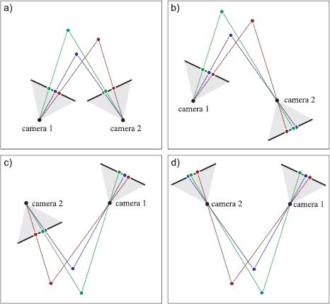
Figure 16.4 Fourfold ambiguity of reconstruction from two pinhole cameras. The mathematical model for the pinhole camera does not distinguish between points that are in front of and points that are behind the camera. This leads to a fourfold ambiguity when we extract the rotation Ω and translation τ relating the cameras from the essential matrix. a) Correct solution. Points are in front of both cameras. b) Incorrect solution. The images are identical, but with this interpretation the points are behind camera 2. c) Incorrect solution with points behind camera 1. d) Incorrect solution with points behind both cameras.
16.3 The fundamental matrix
The derivation of the essential matrix in Section 16.2 used normalized cameras (where Λ1 = Λ2 = I). The fundamental matrix plays the role of the essential matrix for cameras with arbitrary intrinsic matrices Λ1 and Λ2. The general projection equations for the two cameras are
![]()
and we can use similar manipulations to those presented in Section 16.2 to derive the constraint
![]()
or
![]()
where the 3 × 3 matrix F = Λ2-T EΛ1-1 = Λ-T2 τ × ΩΛ-11 is termed the fundamental matrix. Like the essential matrix, it also has rank two, but unlike the essential matrix it has 7 degrees of freedom.
If we know the fundamental matrix F and the intrinsic matrices Λ1 and Λ2, it is possible to recover the essential matrix E using the relation
![]()
and this can further be decomposed to find the rotation and translation between the cameras using the method of Section 16.2.2. It follows that for calibrated cameras, if we can estimate the fundamental matrix, then we can find the rotation and translation between the cameras. Hence, we now turn our attention on how to compute the fundamental matrix.
16.3.1 Estimation of the fundamental matrix
The fundamental matrix relation (Equation 16.22) is a constraint on the possible positions of corresponding points in the first and second images. This constraint is parameterized by the nine entries of F. It follows that if we analyze a set of corresponding points, we can observe how they are constrained, and from this we can deduce the entries of the fundamental matrix F.
A suitable cost function for the fundamental matrix can be found by considering the epipolar lines. Consider a pair of matching points {xi1, xi2} in images 1 and 2, respectively. Each point induces an epipolar line in the other image: the point xi1 induces line li2 in image 2 and the point xi2 induces the line li1 in image 1. When the fundamental matrix is correct, each point should lie exactly on the epipolar line induced by the corresponding point in the other image (Figure 16.5). We hence minimize the squared distance between every point and the epipolar line predicted by its match in the other image so that
![]()
where the distance between a 2D point x = [x,y]T and a line l = [a,b,c] is
![]()
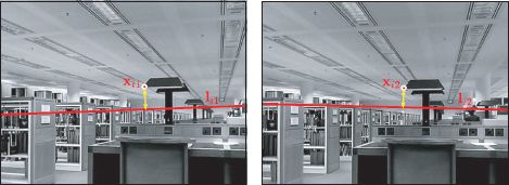
Figure 16.5 Cost function for estimating fundamental matrix. The point xi1 in image 1 induces the epipolar line li2 in image 2. When the fundamental matrix is correct, the matching point xi2 will be on this line. Similarly the point xi2 in image 2 induces the epipolar line li1 in image 1. When the fundamental matrix is correct, the point xi1 will be on this line. The cost function is the sum of the squares of the distances between these epipolar lines and points (yellow arrows). This is termed symmetric epipolar distance.
Here too, it is not possible to find the minimum of Equation 16.24 in closed form, and we must rely on nonlinear optimization methods. It is possible to get a good starting point for this optimization using the eight-point algorithm.
16.3.2 The eight-point algorithm
The eight-point algorithm converts the corresponding 2D points to homogeneous coordinates and then solves for the fundamental matrix in closed form. It does not directly optimize the cost function in Equation 16.24, but instead minimizes an algebraic error. However, the solution to this problem is usually very close to the value that optimizes the desired cost function.
In homogeneous coordinates, the relationship between the ith point xi1 = [xi1, yi1]T in image 1 and the ith point xi2 = [xi2, yi2]T in image 2 is
![]()
where fpq represents one of the entries in the fundamental matrix. When we write this constraint out in full, we get
![]()
This can be expressed as an inner product
![]()
where f = [f11, f12, f13, f21, f22, f23, f31, f32, f33]T is a vectorized version of the fundamental matrix, F.
This provides one linear constraint on the elements of F. Consequently, given I matching points, we can stack these constraints to form the system
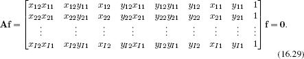
Since the elements of f are ambiguous up to scale, we solve this system with the constraint that |f|=1. This also avoids the trivial solution f = 0. This is a minimum direction problem (see Appendix C.7.2). The solution can be found by taking the singular value decomposition, A=ULVT and setting f to be the last column of V. The matrix F is then formed by reshaping F to form a 3 × 3 matrix.
There are 8 degrees of freedom in the fundamental matrix (it is ambiguous with respect to scale) and so we require a minimum of I = 8 pairs of points. For this reason, this algorithm is called the eight-point algorithm.
In practice, there are several further concerns in implementing this algorithm:
• Since the data are noisy, the singularity constraint of the resulting fundamental matrix will not be obeyed in general (i.e., the estimated matrix will be full rank, not rank two). We reintroduce this constraint by taking the singular decomposition of F, setting the last singular value to zero, and multiplying the terms back out. This provides the closest singular matrix under a Frobenius norm.
• Equation 16.29 is badly scaled since some terms are on the order of pixels squared (~ 10000) and some are of the order ~ 1. To improve the quality of the solution, it is wise to prenormalize the data (see Hartley 1997). We transform the points in image 1 as ![]() ′i1 = T1
′i1 = T1![]() i1 and the points in image 2 as
i1 and the points in image 2 as ![]() ′i2 = T2
′i2 = T2![]() i2. The transformations T1 and T2 are chosen to map the mean of the points in their respective image to zero, and to ensure that the variance in the x- and y-dimensions is one. We then compute the matrix F′ from the transformed data using the eight-point algorithm, and recover the original fundamental matrix as F = TT2 F′ T1.
i2. The transformations T1 and T2 are chosen to map the mean of the points in their respective image to zero, and to ensure that the variance in the x- and y-dimensions is one. We then compute the matrix F′ from the transformed data using the eight-point algorithm, and recover the original fundamental matrix as F = TT2 F′ T1.
• The algorithm will only work if the three-dimensional positions wi corresponding to the eight pairs of points xi1, xi2 are in general position. For example, if they all fall on a plane then the equations become degenerate, and we cannot get a unique solution; here the relation between the points in the two images is given by a homography (see Chapter 15). Similarly, in the case where there is no translation (i.e., τ = 0), the relation between the two images is a homography, and there is no unique solution for the fundamental matrix.
• In the subsequent nonlinear optimization, we must also ensure that the rank of F is two. In order to do this, it is usual to reparameterize the fundamental matrix to ensure that this will be the case.
16.4 Two-view reconstruction pipeline
We now put all of these ideas together and present a rudimentary pipeline for the reconstruction of a static 3D scene based on two images taken from unknown positions, but with cameras where we know the intrinsic parameters. We apply the following steps (Figures 16.6 and 16.7).
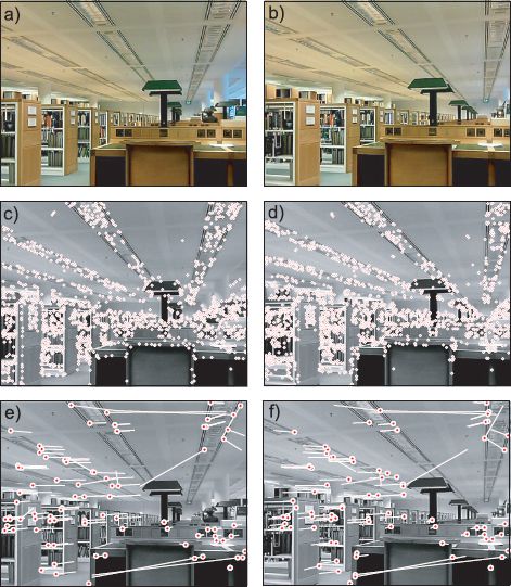
Figure 16.6 Two-view reconstruction pipeline (steps 1-3). a-b) A pair of images of a static scene, captured from two slightly different positions. c-d) SIFT features are computed in each image. A region descriptor is calculated for each feature point that provides a low dimensional characterization of the region around the point. Points in the left and right images are matched using a greedy procedure; the pair of points for which the region descriptors are most similar in a least squares sense are chosen first. Then the pair of remaining points for which the descriptors are most similar are chosen, and so on. This continues until the minimum squared distance between the descriptors exceeds a threshold. e-f) Results of greedy matching procedure: the lines represent the offset to the matching point. Most matches are correct, but there are clearly also some outliers.
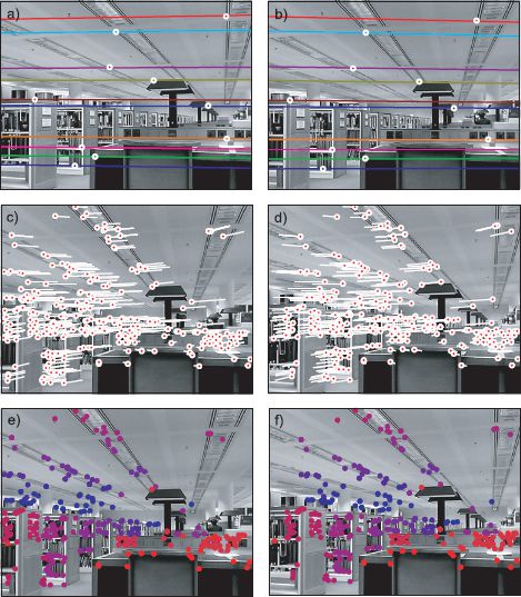
Figure 16.7 Two-view reconstruction pipeline (steps 4-8). A fundamental matrix is fitted using a robust estimation procedure such as RANSAC. a-b) Eight matches with maximum agreement from the rest of the data. For each feature, the epipolar line is plotted in the other image. In each case, the matching point lies on or very near the epipolar line. The resulting fundamental matrix can be decomposed to get estimates for the relative rotation and translation between the cameras. c-d) Result of greedily matching original feature points taking into account the epipolar geometry. Matches where the symmetric epipolar distance exceeds a threshold are rejected. e-f) Computed w coordinate (depth) relative to first camera for each feature. Red features are closer, and blue features are further away. Almost all of the distances agree with our perceived understanding of the scene.
1. Compute image features. We find salient points in each image using an interest point detector such as the SIFT detector (Section 13.2.3).
2. Compute feature descriptors. We characterize the region around each feature in each image with a low-dimensional vector. One possibility would be to use the SIFT descriptor (Section 13.3.2).
3. Find initial matches. We greedily match features between the two images. For example, we might base this on the squared distance between their region descriptors and stop this procedure when the squared distance exceeds a predefined threshold to minimize false matches. We might also reject points where the ratio between the quality of the best and second best match in the other image is too close to one (suggesting that alternative matches are plausible).
4. Compute fundamental matrix. We compute the fundamental matrix using the eight-point algorithm. Since some matches are likely to be incorrect, we use a robust estimation procedure such as RANSAC (Section 15.6).
5. Refine matches. We again greedily match features, but this time we exploit our knowledge of the epipolar geometry: if a putative match is not close to the induced epipolar line, it is rejected. We recompute the fundamental matrix based on all of the remaining point matches.
6. Estimate essential matrix. We estimate the essential matrix from the fundamental matrix using Equation 16.23.
7. Decompose essential matrix. We extract estimates of the rotation and translation between the cameras (i.e., the extrinsic parameters) by decomposing the essential matrix (Section 16.2.2). This provides four possible solutions.
8. Estimate 3D points. For each solution, we reconstruct the 3D position of the points using the linear solution from Section 14.6%. We retain the extrinsic parameters where most of the reconstructed points are in front of both cameras.
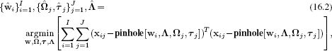
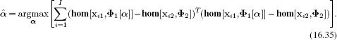
After this procedure, we have a set of I points {xi1}Ii=1 in the first image, a set of I corresponding points {xi2}Ii=1 in the second image, and a good initial estimate of the 3D world positions {wi}Ii=1 that were responsible for them. We also have initial estimates of the extrinsic parameters {Ω,τ}. We now optimize the true cost function
to refine these estimates. In doing so, we must ensure to enforce the constraints that |τ| = 1 and Ω is a valid rotation matrix (see Appendix B).
16.4.1 Minimal solutions
The pipeline described previously is rather naïve; in practice the fundamental and essential matrices can be estimated considerably more efficiently.
For example, the fundamental matrix contains seven degrees of freedom, and so it is actually possible to solve for it using only seven pairs of points. Unsurprisingly, this is known as the seven point algorithm. It is is more complex as it relies on the seven linear constraints and the nonlinear constraint [F] = 0. However, a robust solution can be computed much more efficiently using RANSAC if only seven points are required.
Even if we use this seven-point algorithm, it is still inefficient. When we know the intrinsic parameters of the cameras, it is possible to compute the essential matrix (and hence the relative orientation of the cameras) using a minimal five-point solution. This is based on five linear constraints from observed corresponding points and the nonlinear constraints relating the nine parameters of the essential matrix (Equation 16.12). This method has the advantages of being much quicker to estimate in the context of a RANSAC algorithm and being robust to non-general configurations of the scene points.
16.5 Rectification
The preceding procedure provides a set of sparse matches between the two images. These may suffice for some tasks such as navigation, but if we wish to build an accurate model of the scene, we need to estimate the depth at every point in the image. This is known as dense stereo reconstruction.
Dense stereo reconstruction algorithms (see Sections 11.8.2 and 12.8.3) generally assume that the corresponding point lies on the same horizontal scanline in the other image. The goal of rectification is to preprocess the image pair so that this is true. In other words, we will transform the images so that each epipolar line is horizontal and so that the epipolar lines associated with a point fall on the same scanline to that point in the other image. We will describe two different approaches to this problem.
16.5.1 Planar rectification
We note that the epipolar lines are naturally horizontal and aligned when the camera motion is purely horizontal and both image planes are perpendicular to the w-axis (Figure 16.3a). The key idea of planar rectification is to manipulate the two images to recreate these viewing conditions. We apply homographies Φ1 and Φ2 to the two images so that they cut their respective ray bundles in the desired way (Figure 16.8).
In fact there is an entire family of homographies that accomplish this goal. One possible way to select a suitable pair is to first work with image 2. We apply a series of transformations Φ = T3T2T1, which collectively move the epipole e2 to a position at infinity [1,0,0]T.
We first center the coordinate system on the principal point,
![]()
Then we rotate the image about this center until the epipole lies on the x-axis,
![]()
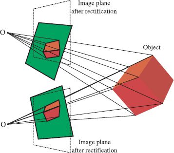
Figure 16.8 Planar rectification. Green quadrilaterals represent image planes of two cameras viewing a 3D object (cube). The goal of planar rectification is to transform each of these planes so that the final configuration replicates Figure 16.3a. After this transformation (dotted lines), the image planes are coplanar, and the translation between the cameras is parallel to this plane. Now the epipolar lines are horizontal and aligned. Since the transformed planes are just different cuts through the respective ray bundles, each transformation can be accomplished using a homography.
where θ = atan2[ey,ex] is the angle of the translated epipole e = [ex,ey]. Finally, we translate the epipole to infinity, using the transformation
![]()
where ex is the x-coordinate of the epipole after the previous two transformations.
After these transformations, the epipole in the second image is at infinity in the horizontal direction. The epipolar lines in this image must converge at the epipole, and are consequently parallel and horizontal as desired.
Now we consider the first image. We cannot simply apply the same procedure as this will not guarantee that the epipolar lines in the first image will be aligned with those in the first. It transpires, however, that there is a family of possible transformations that do make the epipolar lines of this image horizontal and aligned with those in the second image. This family can (not obviously) be parameterized as
![]()
where e2 = [1,0,0]T is the transformed epipole in the second image, and α = [α1,α2,α3]T is a 3D vector that selects the particular transformation from the family. The matrix M comes from the decomposition of the fundamental matrix into F = SM, where S is skew symmetric (see below). A proof of the relation in Equation 16.34 can be found in Hartley and Zisserman (2004).
A sensible criterion is to choose α so that it minimizes the disparity,
This criterion simplifies to solving the least squares problem |Aα-b|2 where
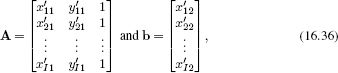
where the vectors x′ij = [x′ij, y′ij]T are defined by
![]()
This least squares problem can be solved using the standard approach (Appendix C.7.1). Figure 16.9 shows example rectified images. After these transformations, the corresponding points are guaranteed to be on the same horizontal scanline, and dense stereo reconstruction can proceed.
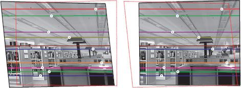
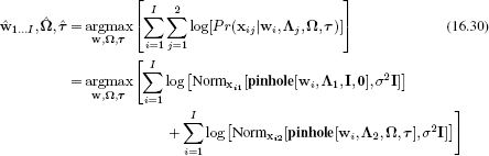
Figure 16.9 Planar rectification. The images from Figures 16.6 and 16.7 have been rectified by applying homographies. After rectification, each point induces an epipolar line in the other image that is horizontal and on the same scanline (compare to Figure 16.7a). This means that the match is guaranteed to be on the same scanline. In this figure, the red dotted line is the superimposed outline of the other image.
Decomposition of the fundamental matrix
The preceding algorithm requires the matrix M from the decomposition of the fundamental matrix as F = SM, where S is skew symmetric. A suitable way to do this is to compute the singular value decomposition of the fundamental matrix F = ULVT. We then define the matrices.
![]()
where lii denotes the ith element from the diagonal of L. Finally, we choose
![]()
16.5.2 Polar rectification
The planar rectification method described in Section 16.5.1 is suitable when the epipole is sufficiently far outside the image. Since the basis of this method is to map the epipoles to infinity, it cannot work when the epipole is inside the image and distorts the image a great deal if it is close to the image. Under these circumstances, a polar rectification is preferred.
Polar rectification applies a nonlinear warp to each image so that corresponding points are mapped to the same scanline. Each new image is formed by resampling the original images so that the first new axis is the distance from the epipole and the second new axis is the angle from the epipole (Figure 16.10). This approach can distort the image significantly but works for all camera configurations.
This method is conceptually simple but should be implemented with caution; when the epipole lies within the camera image, it is important to ensure that the correct half of the epipolar line is aligned with the appropriate part of the other image. The reader is encouraged to consult the original description (Pollefeys et al. 1999b) before implementing this algorithm.
16.5.3 After rectification
After rectification, the horizontal offset between every point in the first image and its corresponding point in the second image can be computed using a dense stereo algorithm (see Sections(see Sections 11.8.2 and 12.8.3). Typical results are shown in Figure 16.11. Each point and its match are then warped back to their original positions (i.e., their image positions are “un-rectified”). For each pair of 2D points, the depth can then be computed using the algorithm of Section 14.6.
Finally, we may wish to view the model from a novel direction. For the two-view case, a simple way to do this is to form a 3D triangular mesh and to texture this mesh using the information from one or the other image. If we have computed dense matches using a stereo-matching algorithm, then the mesh can be computed from the perspective of one camera with two triangles per pixel and cut where there are sharp depth discontinuities. If we have only a sparse correspondence between the two images, then it is usual to triangulate the projections of the 3D points in one image using a technique such as Delaunay triangulation to form the mesh. The textured mesh can now be viewed from a novel direction using the standard computer graphics pipeline.
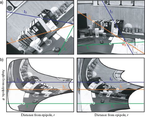
Figure 16.10 Polar rectification. When the epipole is inside one of the images, the planar rectification method is no longer suitable. An alternative in this situation is to perform a nonlinear warp of each image, in which the two new dimensions correspond to the distance and angle from the epipole, respectively. This is known as polar rectification.
16.6 Multiview reconstruction
So far, we have considered reconstruction based on two views of a scene. Of course, it is common to have more than two views. For example, we might want to build 3D models using a video sequence taken by a single moving camera, or equivalently from a video sequence from a static camera of a rigidly moving object (Figure 16.12). This problem is often referred to as structure from motion or multiview reconstruction.
The problem is conceptually very similar to the two camera case. Once again, the solution ultimately relies on a nonlinear optimization in which we manipulate the camera position and the three-dimensional points to minimize the squared reprojection error (Equation 16.2), and hence maximize the likelihood of the model. However, the multiview case does bring several new aspects to the problem.
First, if we have a number of frames all taken with the same camera, there are now sufficient constraints to estimate the intrinsic parameters as well. We initialize the camera matrix with sensible values and add this to the final optimization. This process is known as auto-calibration. Second, matching points in video footage is easier because the changes between adjacent frames tend to be small, and so the features can be explicitly tracked in two dimensions. However, it is usual for some points to be occluded in any given frame, so we must keep track of which points are present at which time (Figure 16.12f).
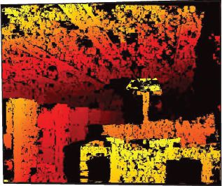
Figure 16.11 Disparity. After rectification, the horizontal offset at each point can be computed using a dense stereo algorithm. Here we used the method of Sizintsev et al. (2010). Color indicates the horizontal shift (disparity) between images. Black regions indicate places where the matching was ambiguous or where the corresponding part of the scene was occluded. Given these horizontal correspondences, we undo the rectification to get a dense set of matching points with 2D offsets. The 3D position can now be computed using the method from Section 14.6.
Third, there are now additional constraints on feature matching, which make it easier to eliminate outliers in the matching set of points. Consider a point that is matched between three frames. The point in the third frame will be constrained to lie on an epipolar line due to the first frame and another epipolar line due to the second frame: its position has to be at the intersection of the two lines and so is determined exactly. Unfortunately, this method will not work when the two predicted epipolar lines are the same as there is not a unique intersection. Consequently, the position in the third view is computed in a different way in practice. Just as we derived the fundamental matrix relation (Equation 16.22) constraining the positions of matching points between two views, it is possible to derive a closed-form relation that constrains the positions across three images. The three-view analogue of the fundamental matrix is called the tri-focal tensor. It can be used to predict the position of the point in a third image given its position in the first and second images even when the epipolar lines are parallel. There is also a relation between four images, which is captured by the quadri-focal tensor, but there are no further relations between points in J > 5 images.
Finally, there are new ways to get initial estimates of the unknown quantities. It may not be practical to get the initial estimates of camera position by computing the transformation between adjacent frames and chaining these through the sequence. The translation between adjacent frames may be too small to reliably estimate the motion, and errors accrue as we move through the sequence. Moreover, it is difficult to maintain a consistent estimate of the (ambiguous) scale throughout. To this end, methods have been developed that simultaneously provide an initial estimate of all the camera positions and 3D points, some of which are based on factorization of a matrix containing all the (x,y) positions of every point tracked throughout the sequence.
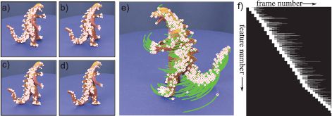
Figure 16.12 Multiframe structure from motion. The goal is to construct a 3D model from a continuous video stream of a moving camera viewing a static object, or a static camera viewing a moving rigid object. a-d) Features are computed in each frame and tracked through t e sequence. e) Features in current frame and their history. f) In each new frame a number of new features is identified, and these are tracked until they are occluded or the correspondence is lost. Here, the white pixels indicate that a feature was present in a frame, and black pixels indicate that it was absent.
16.6.1 Bundle adjustment
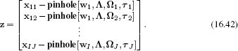
After finding the initial estimates of the 3D positions (structure) and the camera positions (motion), we must again resort to a large nonlinear optimization problem to fine-tune these parameters. With I tracked points over J frames, the problem is formulated as
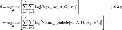
where θ contains the unknown world points {wi}Ii = 1, the intrinsic matrix Λ, and the extrinsic parameters {Ωj, Tj}Jj = 1. This optimization problem is known as Euclidean bundle adjustment. As for the two-view case, it is necessary to constrain the overall scale of the solution in some way.
One way to solve this optimization problem is to use an alternating approach. We first improve the log likelihood with respect to each of the extrinsic sets of parameters {Ωj, τj} (and possibly the intrinsic matrix Λ if unknown) and then update each 3D position wi. This is known as resection-intersection. It seems attractive as it only involves optimizing over a small subset of parameters at any one time. However, this type of coordinate ascent is inefficient: it cannot take advantage of the large gains that come from varying all of the parameters at once.
To make progress, we note that the cost function is based on the normal distribution and so can be rewritten in the least squares form
![]()
where the vector z contains the squared differences between the observed feature positions xij and the positions pinhole[wi,Λ,Ωj,τj] predicted by the model with the current parameters:
The Gauss-Newton method (Appendix B.2.3) is specialized to this type of problem and updates the current estimate θ[t] of the parameters using
![]()
where J is the Jacobian matrix. The entry in the mth row and nth column of J consists of the derivative of the mth element of z with respect to the nth element of the parameter vector θ:
![]()
In a real structure from motion problem, there might be thousands of scene points, each with three unknowns, and also thousands of camera positions, each with six unknowns. At each stage of the optimization, we must invert JTJ, which is a square matrix whose dimension is the same as the number of unknowns. When the number of unknowns is large, inverting this matrix becomes expensive.
However, it is possible to build a practical system by exploiting the sparse structure of JTJ. This sparsity results from the fact that every squared error term does not depend on every unknown. There is one contributing error term per observed 2D point, and this depends only on the associated 3D point, the intrinsic parameters, and the camera position in that frame.
To exploit this structure, we order the elements of the Jacobian matrix as J = [Jw, JΩ], where Jw contains the terms that relate to the unknown world points {wi}Ii = 1 in turn, and JΩ contains the terms that relate to the unknown camera positions {Ωj,Tj}Jj = 1. For pedagogical reasons, we will assume that the intrinsic matrix Λ is known here and hence has no entries in the Jacobian. We see that the matrix to be inverted becomes
![]()
We now note that the matrices in the top-left and bottom-right of this matrix are block-diagonal (different world points do not interact with one another, and neither do the parameters from different cameras). Hence, these two submatrices can be inverted very efficiently. The Schur complement relation (Appendix C.8.2), allows us to exploit this fact to reduce the complexity of the larger matrix inversion.
The preceding description is only a sketch of a real bundle adjustment algorithm; in a real system, additional sparseness in JTJ would be exploited, a more sophisticated optimization method such as Levenberg-Marquardt would be employed, and a robust cost function would be used to reduce the effect of outliers.
16.7 Applications
We first describe a typical pipeline for recovering a 3D mesh model from a sequence of video frames. We then discuss a system that can extract 3D information about a scene from images gathered by a search engine on the Internet, and use this information to help navigate through the set of photos. Finally, we discuss a multicamera system for capturing 3D objects that uses a volumetric representation and exploits a Markov random field prior to get a smooth reconstruction.
16.7.1 3D reconstruction pipeline
Pollefeys and Van Gool (2002) present a complete pipeline for constructing 3D models from a sequence of images taken from an uncalibrated hand-held camera (Figure 16.13). In the first stage, they compute a set of interest points (corners) in each image. When the image data consist of individual still photos, these points are matched between images. When the image data consist of continuous video, they are tracked between frames. In either case, a sparse set of potential correspondences is obtained. The multiview relations are estimated using a robust procedure, and these are then used to eliminate outliers from the correspondence set.
To estimate the motion of the cameras, two images are chosen, and a projective reconstruction is computed (i.e., a reconstruction that is ambiguous up to a 3D projective transformation because the intrinsic parameters are not known). For each of the other images in turn, the pose for the camera is determined relative to this reconstruction, and the reconstruction is refined. In this way, it is possible to incorporate views that have no common features with the original two frames.
A subsequent bundle adjustment procedure minimizes the reprojection errors to get more accurate estimates of the camera positions and the points in the 3D world. At this stage, the reconstruction is still ambiguous up to a projective ambiguity and only now are initial estimates of the intrinsic parameters computed using a specialized procedure (see Pollefeys et al. 1999a). Finally, a full bundle adjustment method is applied; it simultaneously refines the estimates of the intrinsic parameters, camera positions, and 3D structure of the scene.
Successive pairs of images are rectified, and a dense set of disparities are computed using a multiresolution dynamic programming technique. Given these dense correspondences, it is possible to compute an estimate of the 3D scene from the point of view of both cameras. A final estimate of the 3D structure relative to a reference frame is computed by fusing all of these independent estimates using a Kalman filter (see Chapter 19).
For relatively simple scenes, a 3D mesh is computed by placing the vertices of the triangles in 3D space according to the values found in the depth map of the reference frame. The associated texture map can be retrieved from one or more of the original images. For more complex scenes, a single reference frame may not suffice and so several meshes are computed from different reference frames and fused together. Figures 16.13g-h show examples of the resulting textured 3D model of a Medusa head at the ancient site of Sagalassos in Turkey. More details concerning this pipeline can be found in Pollefeys et al. (2004).
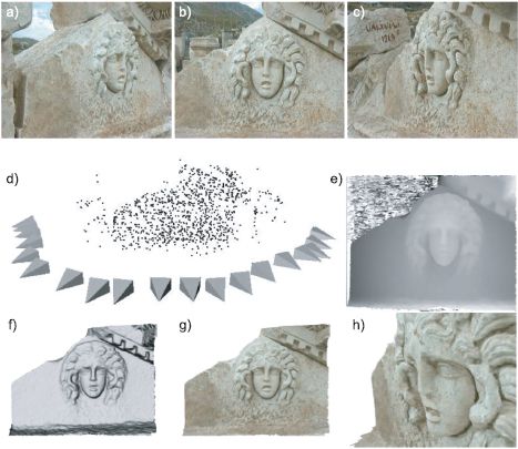
Figure 16.13 3D reconstruction pipeline. a-c) A 20-second video sequence of the camera panning around the Medusa carving was captured. Every 20th frame was used for the reconstruction, three of which are shown here. d) Sparse reconstruction (points) and estimated camera positions (pyramids) after bundle adjustment procedure. e) Depth map after dense stereo matching. f) Shaded 3D mesh model. g-h) Two views of textured 3D mesh model. Adapted from Pollefeys and Van Gool (2002). ©2002 Wiley.
16.7.2 Photo-tourism
Snavely et al. (2006) present a system for browsing a collection of images of an object that were gathered from the Internet. A sparse 3D model of the object is created by locating SIFT features in each image and finding a set of correspondences between pairs of images by computing the fundamental matrix using the eight point algorithm with RANSAC.
A bundle adjustment procedure is then applied to estimate the camera positions and a sparse 3D model of the scene (Figure 16.14a). This optimization procedure starts with only a single pair of images and gradually includes images based on their overlap with the current reconstruction, “rebundling” at each stage. The intrinsic matrix of each camera is also estimated in this step, but this is simplified by assuming that the center of projection is coincident with the image center, that the skew is zero, and that the pixels are square, leaving a single focal length parameter. This is initialized in the optimization using information from the tags of the image when they are present. The bundle adjustment procedure was lengthy; for the model of NotreDame, it took two weeks to compute a model from 2635 photos of which 597 images were ultimately included. However, more recent approaches to reconstruction from Internet photos such as that of Frahm et al. (2010) are considerably faster.
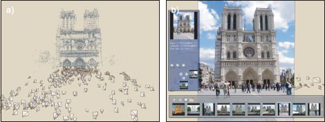
Figure 16.14 Photo-tourism. a) A sparse 3D model of an object is computed from a set of photographs retrieved from the Internet and the relative positions of the cameras (pyramids) are estimated. b) This 3D model is used as the basis of an interface that provides novel ways to explore the photo-collection by moving from image to image in 3D space. Adapted from Snavely et al. (2006). ©2006 ACM.
This sparse 3D model of the scene is exploited to create a set of tools for navigating around the set of photographs. For example, it is possible to
• Select a particular view based on a 3D rendering (as in Figure 16.14a),
• Find images of the object that are similar to the current view,
• Retrieve images of the object taken from the left or the right of the current position (effectively pan around the object),
• Find images that are from a similar viewpoint but closer or further from the object (zoom into/away from the object),
• Annotate objects and have these annotations transferred to other images.
This system was extended by Snavely et al. (2008) to allow more natural interaction with the space of images. For example, in this system it is possible to pan smoothly around objects by warping the original photos, so that they appear to define a smooth path through space.
16.7.3 Volumetric graph cuts
The reconstruction pipeline described in Section 16.7.1 has the potential disadvantage that it requires the merging of multiple meshes of the object computed from different viewpoints. Vogiatzis et al. (2007) presented a system that uses a volumetric representation of depth to avoid this problem. In other words, the 3D space that we wish to reconstruct is divided into a 3D grid, and each constituent element (voxel) is simply labeled as being inside or outside the object. Hence, reconstruction can be viewed as a binary segmentation of the 3D space.
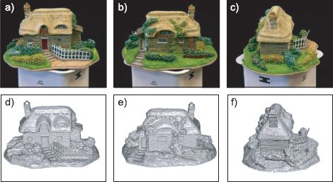
Figure 16.15 Volumetric graph cuts. a-c) Three of the original photos used to build the 3D model. d-f) Renderings of the resulting model from similar viewpoints. Adapted from Vogiatzis et al. (2007). ©2007 IEEE.
The relative positions of the cameras are computed using a standard bundle adjustment approach. However, the reconstruction problem is now formulated in terms of an energy function consisting of two terms and optimized using graph cuts. First, there is an occupation cost for labeling each voxel as either foreground or background. Second, there is a discontinuity cost for lying at the boundary between the two partitions. We will now examine each of these terms in more detail.
The cost of labeling a voxel as being within the object is set to a very high value if this voxel does not project into the silhouette of the object in each image (i.e., it is not within the visual hull). Conversely, it is assumed that concavities in the object do not extend beyond a fixed distance from this visual hull, so a very high cost is paid if voxels close to the center of the visual hull are labeled as being outside the object. For the remaining voxels, a data-independent cost is set that favors the voxel being part of the object and produces a ballooning tendency that counters the shrinking bias of the graph cut solution, which pays a cost at transitions between the object and the space around it.
The discontinuity cost for lying on the boundary of the object depends on the photo-consistency of the voxel; a voxel is deemed photo-consistent if it projects to positions with similar RGB values in all of the cameras from which it is visible. Of course, to evaluate this, we must estimate the set of cameras in which this point is visible. One approach to this is to approximate the shape of the object using the visual hull. However, Vogiatzis et al. (2007) propose a more sophisticated method in which each camera votes for the photo-consistency of the voxel based on its pattern of correlation with the other images.
The final optimization problem now takes the form of a sum of unary occupation costs and pairwise terms that encourage the final voxel label field to be smooth. These pairwise terms are modified by the discontinuity cost (an example of using geodesic distance in graph cuts) so that the transition from foreground to background is more likely in regions where the photo-consistency is high. Figure 16.15 shows an example of a volumetric 3D model computed in this way.
Discussion
This chapter has not introduced any truly new models; rather we have explored the ramifications of using multiple projective pinhole camera models simultaneously. It is now possible to use these ideas to reconstruct 3D models from camera sequences of rigid objects with well-behaved optical properties. However, 3D reconstruction in more general cases remains an open research problem.
Notes
Multiview geometry: For more information about general issues in multiview geometry consult the books by Faugeras et al. (2001), Hartley and Zisserman (2004), and Ma et al. (2004) and the online tutorial by Pollefeys (2002). A summary of multiview relations was presented by Moons (1998).
Essential and fundamental matrices: The essential matrix was described by Longuet-Higgins (1981) and its properties were explored by Huang and Faugeras (1989), Horn (1990), and Maybank (1998) among others. The fundamental matrix was discussed in Faugeras (1992), Faugeras et al. (1992), and Hartley (1992), (1994). The eight-point algorithm for computing the essential matrix is due to Longuet-Higgins (1981). Hartley (1997) described a method for rescaling in the eight-point algorithm that improved its accuracy. Details of the seven-point algorithm for computing the fundamental matrix can be found in Hartley and Zisserman (2004). Nistér (2004) and Stewénius et al. (2006) describe methods for the relative orientation problem that work directly with five-point correspondences between the cameras.
Rectification: The planar rectification algorithm described in the text is adapted from the description in Hartley and Zisserman (2004). Other variations on planar rectification can be found in Fusiello et al. (2000), Loop Zhang (1999), and Ma et al. (2004). The polar rectification procedure is due to Pollefeys et al. (1999b).
Features and feature tracking: The algorithms in this chapter rely on the computation of distinctive points in the image. Typically, these are found using the Harris corner detector Harris corner detector (Harris and Stephens 19888) or the SIFT detector (Lowe 2004). A more detailed discussion of how these points are computed can be found in Section 13.2. Methods for tracking points in smooth video sequences (as opposed to matching them across views with a wide baseline) are discussed in Lucas and Kanade (1981), Tomasi and Kanade (1991), Shi and Tomasi (1994).
Reconstruction pipelines: Several authors have described pipelines for computing 3D structure based on a set of images of a rigid object including Fitzgibbon and Zisserman (1998) Pollefeys et al. (2004), Brown and Lowe (2005), and Agarwal et al. (2009). Newcombe and Davison (2010) present a recent system that runs at interactive speeds. A summary of this area can be found in Moons et al. (2009).
Factorization: Tomasi and Kanade (1992) developed an exact ML solution for the projection matrices and 3D points in a set of images based on factorization. This solution assumes that the projection process is affine (a simplification of the full pinhole model) and that every point is visible in every image. Sturm and Triggs (1996) developed a similar method that could be used for the full projective camera. Buchanan and Fitzgibbon (2005) discuss approaches to this problem when the complete set of data is not available.
Bundle adjustment: Bundle adjustment is a complex topic, which is reviewed in Triggs et al. (1999). More recently Engels et al. (2006) discuss a real-time bundle adjustment approach that works with temporal subwindows from a video sequence. Recent approaches to bundle adjustment have adopted a conjugate gradient optimization strategy (Byröd andÅström 2010; Agarwal et al. 2010). A public implementation of bundle adjustment has been made available by Lourakis and Argyros (2009). A system which is cutting edge at the time of writing is described in Jeong et al. (2010), and recent methods that use multicore processing have also been developed (Wu et al. 2011).
Multiview reconstruction: The stereo algorithms in Chapters 11 and 12 compute an estimate of depth at each pixel of one or both of the input images. An alternative strategy is to use an image-independent representation of shape. Examples of such representations include voxel occupancy grids (Vogiatzis et al. 2007; kutalakos and Seitz 2000), level sets Faugeras and Keriven 1998; Pons et al. 2007), and polygonal meshes (Fua and Leclerc 1995, Hernández and Schmitt 2004). Many multiview reconstruction techniques also enforce the constraints imposed by the silhouettes (see Section 14.7.2) on the final solution (e.g., Sinha and Pollefeys 2005; Sinha et al. 2007; Kolev and Cremers 2008). A review of multiview reconstruction techniques can be found in Seitz et al. (2006).
Problems
16.1 Sketch the pattern of epipolar lines on the images in Figure 16.17a.
16.2 Show that the cross product relation can be written in terms of a matrix multiplication so that
![]()
16.3 Consider Figure 16.16. Write the direction of the three 3D vectors O1O2,O1w, and O2w in terms of the observed image positions x1,x2 and the rotation Ω and translation τ between the cameras. The scale of the vectors is unimportant.
The three vectors that you have found must be coplanar. The criterion for three 3D vectors a, b, c being coplanar can be written as (a × b).c. Use this criterion to derive the essential matrix.
16.4 A clueless computer vision professor writes:
“The essential matrix is a 3 × 3 matrix that relates image coordinates between two images of the same scene. It contains 8 independent degrees of freedom (it is ambiguous up to scale). It has rank 2. If we know the intrinsic matrices of the two cameras, we can use the essential matrix to recover the rotation and translation between the cameras exactly.”
Edit this statement to make it factually correct.
16.5 The essential matrix relates points in two cameras so that
![]()
is given by
![]()
What is the epipolar line in image 2 corresponding to the point x1 = [1,-1, 1]? What is the epipolar line in image 2 corresponding to the points x1 = [-5,-2, 1]? Determine the position of the epipole in image 2. What can you say about the motion of the cameras?
16.6 Show that we can retrieve the essential matrix by multiplying together the expressions from the decomposition (Equations 16.19) as E = τ × Ω.
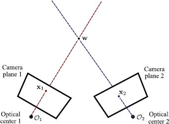
Figure 16.16 Figure for Problem 16.3.
16.7 Derive the fundamental matrix relation:
![]()
16.8 I intend to compute the fundamental matrix using the eight-point algorithm. Unfortunately, my data set is polluted by 30 percent outliers. How many iterations of the RANSAC algorithm will I need to run to have a 99 percent probability of success (i.e., computing the fundamental matrix from eight inliers at least once)? How many iterations will I need if I use an algorithm based on seven points?
16.9 We are given the fundamental matrix F13 relating images 1 and 3 and the fundamental matrix F23 relating images 2 and 3. I am now given corresponding points x1 and x2 in images 1 and 2, respectively. Derive a formula for the position of the corresponding point in image 3.
16.10 Tomasi-Kanade factorization. In the orthographic camera(Figure 14.19), the projection process can be described as
or in matrix form
![]()
Now consider a data matrix X containing the positions {xij}IJi,j=1 of J points as seen in I images so that
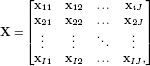
Figure 16.17 a) Figure for Problem 16.1. c) Figure for Problem 16.11. Gray regions represent nonzero entries in this portrait Jacobian matrix.
and where xij=[xij,yij]T.
(i) Show that the matrix X can be written in the form
![]()
where P contains all of the I 3 × 2 projection matrices ![]() , W contains all of the J 3D world positions {wj}Jj=1 and T contains the translation vectors {τ′i}Ii=1.
, W contains all of the J 3D world positions {wj}Jj=1 and T contains the translation vectors {τ′i}Ii=1.
(ii) Devise an algorithm to recover the matrices P, W and T from the measurements X. Is your solution unique?
16.11 Consider a Jacobian that has a structure of nonzero entries as shown in Figure 16.17b. Draw an equivalent image that shows the structure of the nonzero entries in the matrix JTJ. Describe how you would use the Schur complement relation to invert this matrix efficiently.