Computer Vision: Models, Learning, and Inference (2012)

This chapter concerns models for 2D and 3D shape. The motivation for shape models is twofold. First, we may wish to identify exactly which pixels in the scene belong to a given object. One approach to this segmentation problem, is to model the outer contour of the object (i.e., the shape) explicitly. Second, the shape may provide information about the identity or other characteristics of the object: it can be used as an intermediate representation for inferring higher-level properties.

Unfortunately, modeling the shape of an object is challenging; we must account for deformations of the object, the possible absence of some parts of the object and even changes in the object topology. Furthermore, the object may be partially occluded, making it difficult to relate the shape model to the observed data.

One possible approach to establishing 2D object shape is to use a bottom-up approach; here, a set of boundary fragments are identified using an edge detector (Section 13.2.1) and the goal is to connect these fragments to form a coherent object contour. Unfortunately, achieving this goal has proved surprisingly elusive. In practice, the edge detector finds extraneous edge fragments that are not part of the object contour and misses others that are part of the true contour. Hence it is difficult to connect the edge fragments in a way that correctly reconstructs the contour of an object.

The methods in this chapter adopt the top-down approach. Here, we impose prior information about the object that constrains the possible contour shapes and hence reduces the search space. We will investigate a range of different types of prior information; in some models this will be very weak (e.g., the object boundary is smooth) and in others it will be very strong (e.g., the object boundary is a 2D projection of a particular 3D shape).

To motivate these models, consider the problem of fitting a 2D geometric model of the spine to medical imaging data (Figure 17.1). Our goal is to characterize this complex shape with only a few parameters, which could subsequently be used as a basis for diagnosing medical problems. This is challenging because the local edge information in the image is weak. However, in our favor we have very strong prior knowledge about the possible shapes of the spine.

17.1 Shape and its representation

Before we can introduce concrete models for identifying shape in images, we should define exactly what we mean by the word “shape.” A commonly used definition comes from Kendall (1984) who states that shape “is all the geometrical information that remains when location, scale and rotational effects are filtered out from an object.” In other words, the shape consists of whatever geometric information is invariant to a similarity transformation. Depending on the situation, we may generalize this definition to other transformation types such as Euclidean or affine.

We will also need a way to represent the shape. One approach is to directly define an algebraic expression that describes the contour. For example, a conic defines points x = [x,y]^T as lying on the contour if they obey

This family of shapes includes circles, ellipses, parabolas, and hyperbolas, where the choice of shape depends on the parameters θ = {α,β,γ,δ,∊,ζ}

Algebraic models are attractive in that they provide a closed form expression for the contour, but their applicability is extremely limited; it is difficult to define a mathematical expression that describes a family of complex shapes such as the spine in Figure 17.1. It is possible to model complex objects as superimposed collections of geometric primitives like conics, but the resulting models are unwieldy and lose many of the desirable properties of the closed form representation.

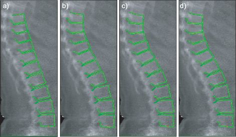
Figure 17.1 Fitting a spine model. a) The spine model is initialized at a fixed position in the image. b-d) The model then adapts to the image until it describes the data as well as possible. Models that “crawl” across the image in this way are known as active shape models. Figure provided by Tim Cootes and Martin Roberts.

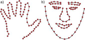
Figure 17.2 Landmark points. Object shape can be represented with sets of landmark points. a) Here the landmark points (red dots) define a single open contour that describes the shape of a hand. b) In this example the landmark points are connected into sets of open and closed contours that describe the regions of the face.

Most of the models in this chapter adopt a different approach; they define the shape using a set of Landmark points (Figure 17.2). One way to think of landmark points is as a set of discrete samples from one or more underlying continuous contours. The connectivity of the landmark points varies according to the model: they may be ordered and hence represent a single continuous contour, ordered with wrapping, so they represent a closed contour or may have a more complex organization so that they can represent a collection of closed and open contours.

The contour can be reconstituted from the landmark points by interpolating between them according to the connectivity. For example, in Figure 17.2, the contours have been formed by connecting adjacent landmark points with straight lines. In more sophisticated schemes, the landmark points may indirectly determine the position of a smooth curve by acting as the control points of a spline model.

17.2 Snakes

As a base model, we will consider parametric contour models, which are sometimes also referred to as active contour models or snakes. These provide only very weak a priori geometric information; they assume that we know the topology of the contour (i.e., open or closed) and that it is smooth but nothing else. Hence they are suitable for situations where little is known about the contents of the image. We will consider a closed contour defined by a set of N2D landmark points W = [w₁, w₂,…,w_N], which are unknown.

Our goal is to find the configuration of landmark points that best explains the shape of an object in the image. We construct a generative model for the landmark positions, which is determined by a likelihood term (which indicates the agreement of this configuration with the image data) and a prior term (which encompasses our prior knowledge about the frequency with which different configurations occur).

The likelihood Pr(x|W) of the RGB image data x given the landmark points W should be high when the landmark points w lie on or close to edges in the image, and low when they lie in flat regions. One possibility for the likelihood is hence

where the function sobel[x,w] returns the magnitude of the Sobel edge operator (i.e., the square root of the sum of the squared responses to the horizontal and vertical Sobel filters - see Section 13.1.3) at 2D position w in the image.

This likelihood will be high when the landmark points are on a contour and low otherwise, as required. However, it has a rather serious disadvantage in practice; in completely flat parts of the image, the Sobel edge operator returns a value of zero. Consequently, if the landmark points lie in flat parts of the image, there is no information about which way to move them to improve the fit (Figures 17.3a-b).

A better approach is to find a set of discrete edges using the Canny edge detector Canny edge detector (Section 13.2.1) and then compute a distance transform; each pixel is allotted a value according to its squared distance from the nearest edge pixel. The likelihood now becomes

where the function [x,w] returns the value of the distance transform at position w in the image. Now the likelihood is large when the landmark points all fall close to edges in the image (where the distance transform is low) and smoothly decreases as the distance between the landmark points and the edges increases (Figures 17.3c-d). In addition to being pragmatic, this approach also has an attractive interpretation; the “squared distance” objective function is equivalent to assuming that the measured position of the edge is a noisy estimate of the true edge position and that the noise is additive and normally distributed.

If we were to find the landmark points W based on this criterion alone, then each point would be separately attracted to a strong edge in the image, and the result would probably not form a coherent shape; they might even all be attracted to the same position. To avoid this problem and complete the model, we define a prior that favors smooth contours with low curvature. There are various ways to do this, but one possibility is to choose a prior with two terms

where the scalars α and β control the relative contribution of these terms.

The first term encourages the spacing of the points around the contour to be even; the function space[w,n] returns a high value if spacing between the n^th contour point w_n and its neighbors is close to the average spacing between neighboring points along the contour:

where we assume that the contour is closed so that w₀ = w_N.

The second term in the prior, curve,[w,n] returns larger values when the curvature is small and so encourages the contour to be smooth. It is defined as

where again we assume that the contour is closed so w₀ = w_N and w_N+1 = w₁.

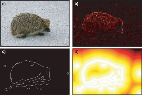
Figure 17.3 Likelihood for landmark points. a) Original image. b) Output of Sobel edge operator - one possible scheme is to assign the landmark points a high likelihood if the Sobel response is strong at their position. This encourages the landmark points to lie on boundaries, in the image but the response is flat in regions away from the boundaries and this makes it difficult to apply gradient methods to fit the model c) Results of applying Canny edge detector. d) Negative distance from nearest Canny edge. This function is also high at boundaries in the image but varies smoothly in regions away from the boundaries.

There are only two parameters in this model (the weighting terms, α and β). These can be learned from training examples, but for simplicity, we will assume that they were set by hand so there is no need for an explicit learning procedure.

17.2.1 Inference

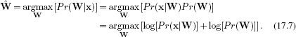
In inference, we observe a new image x and try to fit the points {w_i} on the contour so that they describe the image as well as possible. To this end, we use a maximum a posteriori criterion

The optimum of this objective function cannot be found in closed form, and we must apply a general nonlinear optimization procedure such as the Newton method (Appendix B). The number of unknowns is twice the number of the landmark points as each point has an x and y coordinate.

An example of this fitting procedure is illustrated in Figure 17.4. As the minimization proceeds, the contour crawls around the image, seeking the set of landmark points with highest posterior probability. For this reason, this type of contour model is sometimes known as a snake or active contour model.

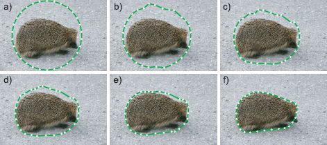
Figure 17.4 Snakes. The snake is defined by a series of connected landmark points. a-f) As the optimization proceeds and the posterior probability of these points increases, the snake contour crawls across the image. The objective function is chosen so that the landmark points are attracted to edges in the image, but also try to remain equidistant from one another and form a shape with low curvature.

The final contour in Figure 17.4 fits snugly around the outer boundary of the hedgehog. However, it has not correctly delineated the nose region; this is an area of high curvature and the scale of the nose is smaller than the distance between adjacent landmark points. The model can be improved by using a likelihood that depends on the image at positions along the contour between the landmark points. In this way, we can develop a model that has few unknowns but that depends on the image in a dense way.

A second problem with this model is that the optimization procedure can get stuck in local optima. One possibility is to restart the optimization from a number of different initial conditions, and choose the final solution with the highest probability. Alternatively, it is possible to modify the prior to make inference more tractable. For example, the spacing term can be redefined as

which encourages the spacing of the points to be close to a predefined value μ_s and hence encourages solutions at a certain scale. This small change makes inference in the model much easier: the prior is now a 1D Markov random field, with cliques that consist of each element and its two neighbors (due to the term in the curve[•,•]). The problem can now be discretized and solved efficiently using dynamic programming methods (see Section 11.8.4).

17.2.2 Problems with the snake model

The simple snake model described previously has a number of limitations; it embodies only weak information about the smoothness of the object boundary and as such:

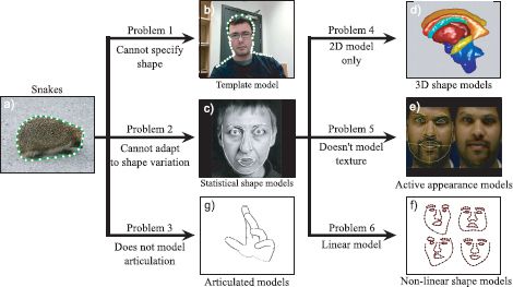
Figure 17.5 Shape models. a) The snake model only assumes that the contour is smooth. b) The template model assumes a priori knowledge of the object shape. c) Active shape models are a compromise in which some information about the object class is known, but the model can adapt to the particular image. d-f) We consider three extensions to the active shape models describe 3D shape, simultaneously model intensity variation, and describe more complex shape variation, respectively. g) Finally, we investigate models in which a priori information about the structure of an articulated object is provided.

• It is not useful where we know the object shape but not its position within the image.

• It is not useful where we know the class of the object (e.g., a face) but not the particular instance (e.g., whose face).

• The snake model is 2D and does not understand that some contours are created by projecting a 3D surface through the camera model.

• It cannot model articulated objects such as the human body.

We remedy these various problems in the subsequent parts of this chapter (Figure 17.5). In Section 17.3, we investigate a model in which we know exactly the shape we are looking for, and the only problem is to find its position in the image. In Sections 17.4-17.8, we investigate models that describe the statistical variation in a class of objects and can find unseen examples of the same class. Finally, in Section 17.9 we discuss articulated models.

17.3 Shape templates

We will now consider shape template models. These impose the strongest possible form of geometric information; it is assumed that we know the shape exactly. So, whereas the snake model started with a circular configuration and adapted this to fit the image, the template model starts with the correct shape of the object and merely tries to identify its position, scale, and orientation in the image. More generally, the problem is to determine the parameters Ψ of the transformation that maps this shape onto the current image.

We will now develop a generative model that determines the likelihood of the observed image data as a function of these transformation parameters. The underlying representation of the shape is again a set W = {w_n}^N_{n = 1} of 2D landmark points, which are now assumed known. However, to explain the observed data, the points must be mapped into the image by a 2D transformation trans[w, Ψ], where Ψ contains the parameters of the transformation model. For example, with a similarity transformation, Ψ would consist of the rotation angle, scaling factor, and 2D translation vector.

As with the snake model, we choose the likelihood of image data x to be dependent on the negative distance from the closest edge in the image

where the function dist[x, w] returns the distance transform of the image x at position w. Again the likelihood is larger when the landmark points all fall in regions where the distance transform is low (i.e., close to edges in the image).

17.3.1 Inference

The only unknown variables in the template model are the transformation parameters Ψ. For simplicity, we will assume that we have no prior knowledge of these parameters and adopt the maximum likelihood approach in which we maximize the log-likelihood L:

There is no closed form solution to this problem, so we must rely on nonlinear optimization. To this end, we must take the derivative of the objective function with respect to the unknowns, and for this we employ the chain rule:

where w′_n = trans[w_n,Ψ] is the transformed point, and w′_jn is the j^th entry in the 2D vector.

The first term on the right-hand side of Equation 17.11 is easy to compute. The derivative of the distance image can be approximated in each direction by evaluating horizontal or vertical derivative filters (Section 13.1.3) at the current position w′_n. In general this will not exactly fall on the center of a pixel and so the derivative values should be interpolated from nearby pixels. The second term depends on the transformation in question.

Figure 17.6 illustrates the fitting procedure for a template model based on an affine transform. As the optimization proceeds, the contour crawls over the image as it tries to find a more optimal position. Unfortunately, there is no guarantee that the optimization will converge to the true position. As for the snake model, one way to deal with this problem is to restart the optimization from many different places and choose the solution with the overall maximum log likelihood. Alternatively, we could initialize the template position more intelligently; in this example the initial position might be based on the output of a face detector. It is also possible to restrict the possible solutions by imposing prior knowledge about the possible transformation parameters and using a maximum a posteriori formulation.

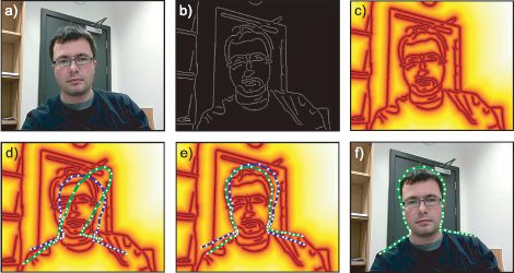
Figure 17.6 Shape templates. Here the shape of the object is known and only the affine transformation relating the shape to the image is unknown. a) Original image. b) Results of applying Canny edge detector. c) Distance transformed image. The intensity represents the distance to the nearest edge. d) Fitting a shape template. The template is initialized with a randomly chosen affine transformation (blue curve). After optimization (green curve) the landmark points, which define the curve, have moved toward positions with lower values in the distance image. In this case, the fitting procedure has converged to a local optimum, and the correct silhouette has not been identified. e) When we start the optimization from nearer the true optimum, it converges to the global maximum. f) Final fit of template.

17.3.2 Inference with iterative closest point algorithm

In Chapter 15 we saw that the transformation mapping one set of points to another can be computed in closed form for several common families of transformations. However, the template model cannot be fit in closed form because we do not know which edge points in the image correspond to each landmark point in the model.

This suggests a different approach to inference for this model. The iterative closest point (ICP) algorithm alternately matches points in the image to the landmark points and computes the best transformation. More precisely:

• Each landmark point w_n is transformed into the image as w′_n = trans[w_n,Ψ] using the current parameters Ψ.

• Each transformed point w′_n is associated with the closest image point y_n that lies on an edge.

• The transformation parameters Ψ that best map the landmark points {w_n}^N_{n = 1} to the image points {y_n}^N_{n = 1} are computed in closed form.

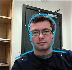
Figure 17.7 Iterative closest point algorithm. We associate each landmark point (positions where the red normals join the blue contour) with a single edge point in the image. In this example, we search along the normal direction to the contour (red lines). There are usually several points identified by an edge detector along each normal (circles). In each case we choose the closest - a process known as data association. We compute the transformation that best maps the landmark points to these closest edge positions. This moves the contour and potentially changes the closest points in the next iteration.

This procedure is repeated until convergence. As the optimization proceeds, the choice of closest points changes - a process known as data association - and so the computed transformation parameters also evolve.

A variation of this approach considers matching the landmark points to edges in a direction that is perpendicular to the contour (Figure 17.7). This means that the search for the nearest edge point is now only in 1D, and this can also make the fitting more robust in some circumstances. This is most practical for smooth contour models where the normals can be computed in closed form.

17.4 Statistical shape models

The template model is useful when we know exactly what the object is. Conversely, the snake model is useful when we have very little prior information about the object. In this section we describe a model that lies in between these two extremes. Statistical shape models, active shape models, or point distribution models describe the variation within a class of objects, and so can adapt to an individual shape from that class even if they have not seen this specific example before.

As with the template and snake models, the shape is described in terms of the positions of the N landmark points {w_n}^N_{n = 1}, and the likelihood of these points depends on their proximity to edges in the image. For example, we might choose the likelihood of the i^th training image data x_i to be

where w_in is the n^th landmark point in the i^th training image and dist[•,•] is a function that computes the distance to the nearest Canny edge in the image.

However, we now define a more sophisticated prior model over the landmark positions, which are characterized as a compound vector w_i = [w^T_i1,w^T_i2…,w^T_iN]^T containing all of the x- and y-positions of the landmark points in the i^th image. In particular, we model the density Pr(w_i) as a normal distribution so that

where the mean μ captures the average shape and the covariance ∑ captures how different instances vary around this mean.

17.4.1 Learning

In learning, our goal is to estimate the parameters θ = {μ,∑} based on training data. Each training example consists of a set of landmark points that have been hand-annotated on one of the training images.

Unfortunately, the training examples are not usually geometrically aligned when we receive them. In other words, we receive the transformed data examples w′_i = [w′^T_i1,w′^T_i2,…,w′^T_iN]^T, where

Before we can learn the parameters μ and ∑ of the normal, we must align the examples using the inverse of this transformation

where are the parameters of the inverse transformations.

Alignment of training examples

The method for aligning the training examples is known as generalized Procrustes analysis (Figure 17.8) and exploits the “chicken and egg” structure of the underlying problem; if we knew the mean shape μ, then it would be easy to estimate the parameters of the transformations that best map the observed points to this mean. Similarly, if we knew these transformations, we could easily compute the mean shape by transforming the observed points and taking the mean of the resulting shapes. Generalized Procrustes analysis takes an alternating approach to this problem in which we repeatedly

1. Update the transformations using the criterion

where μ = [μ^T₁,μ^T₂,…,μ^T_N]^T. This can be achieved in closed form for common transformation families such as the Euclidean, similarity, or affine transformations (see Section 15.2).

2. Update the mean template

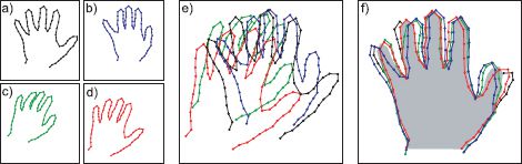
Figure 17.8 Generalized Procrustes analysis. a-d) Four training shapes. e) Superimposing the training shapes shows that they are not aligned well. f) The goal of generalized Procrustes analysis is simultaneously to align all of the training shapes with respect to a chosen transformation family. Here, the images are aligned with respect to a similarity transformation (gray region illustrates mean shape). After this procedure, the remaining variation is described by a statistical shape model.

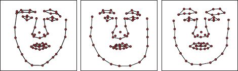
Figure 17.9 Statistical model of face shape. Three samples drawn from normally distributed model of landmark vectors w. Each generated 136-dimensional vector was reshaped to create a 68 × 2 matrix containing 68 (x,y) points, which are plotted in the figure. The samples look like plausible examples of face shapes.

In practice, to optimize this criterion we inversely transform each set of points using Equation 17.15 and take the average of the resulting shape vectors. It is important to normalize the mean vector μ after this stage to define the absolute scale uniquely.

Typically, we would initialize the mean vector μ to be one of the training examples and iterate between these steps until there was no further improvement.

After convergence, we can fit the statistical model

We already know the mean μ. We can compute the covariance ∑ using the maximum likelihood approach from the aligned shapes {w_i}^I_i=1. Figure 17.9 visualizes a shape model for the human face that was learned using this technique.

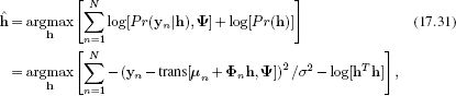
17.4.2 Inference

In inference, we fit the model to a new image. The simplest way to do this is to take a brute force optimization approach in which we estimate the unknown landmark points w = {w_n}^N_n=1 and the parameters Ψ of the transformation model so that

One way to optimize this objective function is to alternate between estimating the transformation parameters and the landmark points. For fixed landmark points {w_n}^N_n=1, we are effectively fitting a shape template model, and we can use the methods of Sections 17.3.1 and 17.3.2 to find the transformation parameters Ψ. For fixed transformation parameters, it is possible to estimate the landmark points by nonlinear optimization of the objective function.

As with the template model, the statistical shape model “crawls” across the image as the optimization discovers improved ways to make the model agree with the image. However, unlike the template model, it can adapt its shape to match the idiosyncrasies of the particular object in this image as in Figure 17.1.

Unfortunately this statistical shape model has some practical disadvantages due to the number of variables involved. In the fitting procedure, we must optimize over the landmark points, themselves. If there are N landmark points, then there are 2N variables over which to optimize. For the face model in Figure 15.9, there would be 136 variables, and the resulting optimization is quite costly. Moreover, we will require a large number of training examples to accurately estimate the covariance ∑ of these variables.

Furthermore, it is not clear that all these parameters are needed; the classes of object that are suited to this normally distributed model (hands, faces, spines, etc.) are quite constrained in their shape variation and so many of the parameters of this full model are merely describing noise in the training shape annotation. In the next section we describe a related model which uses fewer unknown variables (and can be fit more efficiently) and fewer parameters (and so can be learned from less data).

17.5 Subspace shape models

The subspace shape model exploits the structure inherent in the covariance of the landmark points. In particular, it assumes that the shape vectors {w_i}^I_i=1 all lie very close to a K-dimensional linear subspace (see Figure 7.19) and describes the shape vectors as resulting from the process:

where μ is the mean shape, Φ = [₁, ₂,…,_K] is a portrait matrix containing K basis functions {_k}^K_k=1 that define the subspace in its columns, and ∊_i is an additive normal noise term with spherical covariance σ²I. The term h_i is a K×1 hidden variable where each element is responsible for weighting one of the basis functions. This can be seen more clearly by rewriting Equation 17.20 as

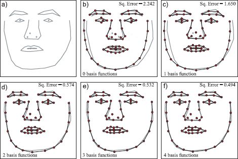
Figure 17.10 Approximation of face by weighting basis functions. a) Original face. b) Approximating original (gray) by mean face μ. c) Approximating original by mean face plus optimal weighting h_i1 of basis function ₁. d-f) Adding further weighted basis functions. As more terms are added, the approximation becomes closer to the original. With only four basis functions, the model can explain 78 percent of the variation of the original face around the mean.

where h_ik is the k^th element of the vector h_i.

The principle of the subspace model is to approximate the shape vector by the deterministic part of this process so that

and so now we can represent the 2N× 1 vector w_i using only the K × 1 vector h_i.

For constrained data sets such as the spine, hand, and face models, it is remarkable how good this approximation can be, even when K is set to quite a small number. For example, in Figure 17.10 the face is very well approximated by taking a weighted sum of only K = 4 basis functions. We will exploit this phenomenon when we fit the shape model; we now optimize over the weights of the basis functions rather than the landmark points themselves, and this results in considerable computational savings.

Of course, the approximation in Figure 17.10 only works because (i) we have selected a set of basis functions Φ that are suitable for representing faces and (ii) we have chosen the weights h_i appropriately to describe this face. We will now take a closer look at the model and how to find these quantities.

17.5.1 Probabilistic principal component analysis

The particular subspace model that we will apply here is known as probabilistic principal component analysis or PPCA for short. To define the model, we reexpress Equation 17.20 in probabilistic terms:

where μ is a 2N × 1 mean vector, Φ is a 2N × K matrix containing K basis functions in its columns, and σ² controls the degree of additive noise. In the context of this model, the basis functions are known as principal components. The K × 1 hidden variable h_i weights the basis functions and determines the final positions on the subspace, before the additive noise component is added.

To complete the model, we also define a prior over the hidden variable h_i, and we choose a spherical normal distribution for this:

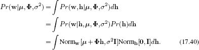
By marginalizing the joint distribution Pr(w_i,h_i) with respect to the hidden variable h_i, we can retrieve the prior density Pr(w_i), and this is given by

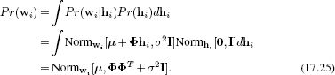
This algebraic result is not obvious; however, it has a simple interpretation. The prior over the landmark points w_i is once more normally distributed, but now the covariance is divided into two parts: the term ΦΦ^T, which explains the variation in the subspace (due to shape changes), and the term σ²I, which explains any remaining variation in the data (mainly noise in the training points).

17.5.2 Learning

The PPCA model is very closely related to factor analysis (Section 7.6). The only difference is that the noise term σ²I is spherical in the PPCA model, but has the diagonal form in factor analysis. Surprisingly, this difference has important implications; it is possible to learn the PPCA model in closed form whereas the factor analysis model needs an iterative strategy such as the EM algorithm.

In learning we are given a set of aligned training data {w_i}^I_i=1 where w_i = [w^T_i1,w^T_i2…,w^T_iN]^T is a vector containing all of the x and y positions of the landmark points in the i^th example. We wish to estimate the parameters μ,Φ, and σ² of the PPCA model.

To this end, we first set the mean parameter μ to be the mean of the training examples w_i:

We then form a matrix W = [w₁ - μ,w₂ - μ,…,w_I - μ] containing the zero-centered data and compute the singular value decomposition of WW^T

where U is an orthogonal matrix and L² is diagonal. For a model that explains D dimensional data with K principal components, we compute the parameters using

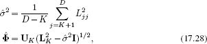
where U_K denotes a truncation of U where we have retained only the first K columns, L²_K represents a truncation of L² to retain only the first K columns and K rows, and L_jj is the j^th element from the diagonal of L.

If the dimensionality D of the data is very high, then the eigenvalue decomposition of the D × D matrix WW^T will be computationally expensive. If the number of training examples I is less than the dimensionality D, then a more efficient approach is to compute the singular value decomposition of the I × I scatter matrix W^TW

and then rearrange the SVD relation W = ULV^T to compute U.

There are two things to notice about the estimated basis functions Φ:

1. The basis functions (principal components) in the columns of Φ are all orthogonal to one another. This can be easily seen because the solution for Φ (Equation 17.28) is the product of the truncated orthogonal matrix U_K and the diagonal matrix .

2. The basis functions are ordered: the first column of Φ represents the direction in the space of w that contained the most variance, and each subsequent direction explains less variation. This is a consequence of the SVD algorithm, which orders the elements of L² so that they decrease.

We could visualize the PPCA model by drawing samples from the marginal density (Equation 17.25). However, the properties of the basis functions permit a more systematic way to examine the model. In Figure 17.11 we visualize the PPCA model by manipulating the hidden variable h_i and then illustrating the vector μ+Φh_i. We can choose h_i to elucidate each basis function {_k}^K_k=1 in turn. For example, by setting h_i= ±[1,0,0,0,…,0] we investigate the first basis function.

Figure 17.11 shows that the principal components _k sometimes have surprisingly clear interpretations. For example, the first principal component clearly encodes the opening and closing of the fingers. A second example that visualizes the spine model from Figure 17.1 is illustrated in Figure 17.12.

17.5.3 Inference

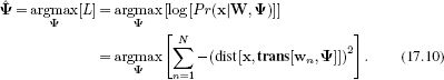
In inference, we fit the shape to a new image by manipulating the weights h of the basis functions Φ. A suitable objective function is

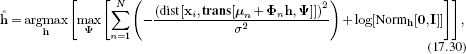
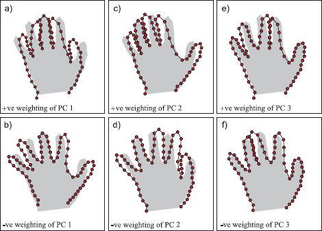
Figure 17.11 Principal components for hand model. a-b) Varying the first principal component. In panel (a) we have added a multiple λ of the first principal component ₁ to the mean vector μ. In panel (b) we have subtracted the same multiple of the first principal component from the mean. In each case the shaded area indicates the mean vector. The first principal component has a clear interpretation: it controls the opening and closing of the fingers. Panels (c-d) and (e-f) show similar manipulations of the second and third principal components, respectively.

where μ_n contains the two elements of μ that pertain to the n^th point and Φ_n contains the two rows of Φ that pertain to the n^th point. There are a number of ways to optimize this model, including a straightforward nonlinear optimization over the unknowns h and Ψ. We will briefly describe an iterative closest point approach. This consists of iteratively repeating these steps:

• The current landmark points are computed as w = μ+Φh.

• Each landmark point is transformed into the image as w′_n = trans[w_n,Ψ].

• Each transformed point w′_n is associated with the closest edge point y_n in the image.

• The transformation parameters Ψ that best map the original landmark points {w_n}^N_n=1 to the edge points {y_n}^N_n=1 are computed.

• Each point is transformed again using the updated parameters Ψ.

• The closest edge points {y_n}^N_n=1 are found once more.

• The hidden variables h are updated (see below).

We repeat these steps until convergence. After optimization, the landmark points can be recovered as w = μ+Φh.

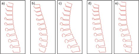
Figure 17.12 Learned spine model. a) Mean spine shape. b-c) Manipulating first principal component. d-e) Manipulating second principal component. Figure provided by Tim Cootes.

In the last step of the iterative algorithm we must update the hidden variables. This can be achieved using the objective function:

where μ_n contains the two elements of μ associated with the n^th landmark point and Φ_n contains the two rows of Φ associated with the n^th landmark point. If the transformation is linear so that trans[w_n,Ψ] can be written in the form Aw_n+b, then this update can be computed in closed form and is given by

Examples of performing inference in subspace shape models are illustrated in Figures 17.1 and 17.13. As the optimization proceeds, the shape model moves across the surface of the image and adapts itself to the shape of the object. For this reason, these models are often referred to as active shape models.

We note that there are many variations of this model and many strategies that help fitting the model robustly. One particularly weak aspect of the model is that it assumes that each landmark point maps to a generic edge in the image; it does not even distinguish between the polarity or orientation of this edge, let alone take advantage of other nearby image information that might help identify the correct position. A more sensible approach is to build a generative model that describes the likelihood of the local image data when the n^th feature w_n is present. A second important concept is coarse-to-fine fitting, in which a coarse model is fitted to a low-resolution image. The result is then used as a starting point for a more detailed model at a higher resolution. In this way, it is possible to increase the probability of converging to the true fit without getting stuck in a local minimum.

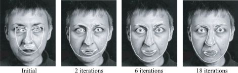
Figure 17.13 Several iterations of fitting a subspace shape model to a face image. After convergence, both the global transformation of the model and the details of the shape are correct. When a statistical shape model is fit to an image in this way, it is referred to as an active shape model. Figure provided by Tim Cootes.

17.6 Three-dimensional shape models

The subspace shape model can be easily extended to three dimensions. For 3D data, the model works in almost exactly the same way as it did in 2D. However, the landmark points w become 3 × 1 vectors determining the position within 3D space, and the global transformation that maps these into the image must also be generalized to 3D. For example, a 3D affine transformation encompasses 3D translations, rotations, shearing, and scaling in 3D and is determined by 12 parameters.

Finally, the likelihood must also be adapted for 3D. A trivial way to do this would be to create the 3D analogue of an edge operator by taking the root mean square of three derivative filters in the coordinate directions. We then construct an expression so that the likelihood is high in regions where the 3D edge operator returns a high value. An example of a 3D shape model is shown in Figure 17.14.

17.7 Statistical models for shape and appearance

In Chapter 7 we discussed the use of subspace models to describe the pixel intensities of a class of images such as faces. However, it was concluded that these were very poor models of this high-dimensional data. In this section, we consider models that describe both the intensity of the pixels and the shape of the object simultaneously. Moreover, they describe correlations between these aspects of the image: the shape tells us something about the intensity values and vice versa (Figure 17.15). When we fit these models to new images, they deform and adapt to the shape and intensity of the image, and so they are known as active appearance models.

As before, we characterize the shape with a vector of N landmark points w = [w^T₁, w^T₂,…, w^T_N]. However, we now also describe a model of the pixel intensity values x where this vector contains the concatenated RGB data from the image. The full model can best be described as a sequence of conditional probability statements:

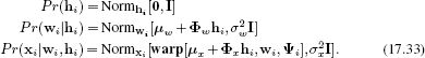
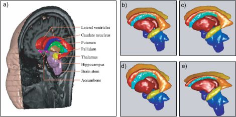
Figure 17.14 Three-dimensional statistical shape model. a) The model describes regions of the human brain. It is again defined by a set of landmark points. These are visualized by triangulating them to form a surface. b-c) Changing the weighting of the first principal component. d-e) Changing weighting of second component. Adapted from Babalola et al. (2008).

Figure 17.15 Modeling both shape and texture. We learn a model in which we a) parameterize shape using a subspace model (results of manipulating weights of shape basis functions shown) and b) parameterize intensity values for fixed shape using a different subspace model (results of manipulating weights of texture basis functions shown). c) The subspace models are connected in that the weightings of the basis functions (principal components) in each model are always the same. In this way, correlations between shape and texture are described (results of manipulating weights of basis functions for both shape and texture together shown). Adapted from Stegmann (2002).

This is quite a complex model, so we will break it down into its constituent parts. At the core of the model is a hidden variable h_i. This can be thought of as a low-dimensional explanation that underpins both the shape and the pixel intensity values. In the first equation, we define a prior over this hidden variable.

In the second equation, the shape data w is created by weighting a set of basis functions Φ_w by the hidden variable and adding a mean vector μ_w. The result is corrupted with spherically distributed normal noise with covariance σ²I. This is exactly the same as for the statistical shape model.

The third equation describes how the observed pixel values x_i in the i^th image depend on the shape w_i, the global transformation parameters Ψ_i and the hidden variable h_i. There are three stages in this process:

1. The intensity values are generated for the mean shape μ_w; pixel values are described as a weighted sum μ_x+Φ_xh_i of a second set of basis functions Φ_x which is added to a mean intensity μ_x.

2. These generated intensity values are then warped to the final desired shape; the operation warp[μ_x+Φ_xh_i,w_i,Ψ_i] warps the resulting intensity image μ_x+Φ_xh_i to the desired shape based on the landmark points w_i and the global transformation parameters Ψ_i.

3. Finally, the observed data x_i is corrupted by normally distributed noise with spherical covariance σ²_xI.

Notice that both the intensity values and the shape depend on the same underlying hidden variable h_i. This means that the model can describe correlations in the shape and appearance; for example, the texture might change to include teeth when the mouth region expands. Figure 17.15 shows examples of manipulating the shape and texture components of a face model and illustrates the correlation between the two. Notice that the resulting images are much sharper than the factor analysis model for faces (Figure 7.22); by explicitly accounting for the shape component, we get a superior model of the texture.

Warping images

A simple approach to warping the images is to triangulate the landmark points and then use a piecewise affine warp; each triangle is warped from the canonical position to the desired final position using a separate affine transformation (Figure 17.16). The coordinates of the canonical triangle vertices are held in μ. The coordinates of the triangle vertices after the warp are held in trans[μ_w+Φ_wh_i,Ψ_i].

17.7.1 Learning

In learning we are given a set of I images in which we know the transformed landmark points {w_i}^I_i=1 and the associated warped and transformed pixel data {x_i}^I_i=1 and we aim to learn the parameters The model is too complex to learn directly; we take the approach of simplifying it by eliminating (i) the effect of the transformation on the landmark points and (ii) both the warp and the transformation on the image data. Then we estimate the parameters in this simplified model.

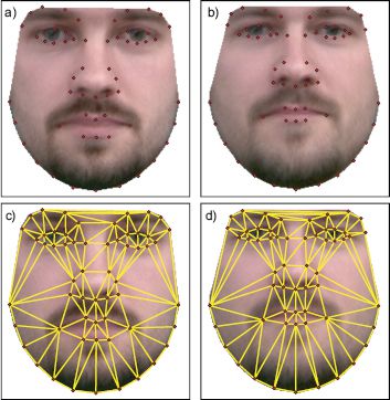
Figure 17.16 Piecewise affine warping. a) The texture is synthesized for a fixed canonical shape. b) This shape is then warped to create the final image. c) One technique for warping the image is to use a piecewise affine transformation. We first triangulate the landmark points. d) Then each triangle undergoes a separate affine transformation such that the three points that define it move to their final positions. Adapted from (2002).

To eliminate the effect of the transformations {Ψ_i}^I_i=1 on the landmark points, we perform generalized Procrustes analysis. To eliminate the effect of the transformation and warps and the observed images, we now warp each training image to the average shape using piecewise affine transformations.

The result of these operations is to generate training data consisting of aligned sets of landmark points {w_i}^I_i=1 representing the shape (similar to Figure 17.15a) and a set of face images {x_i}^I_i=1 that all have the same shape (similar to Figure 17.15b). These data are explained using the simpler model:

To learn the parameters, we write the last two equations in the generative form

where ∊_wi is a normally distributed noise term with spherical covariance σ²_wI and ∊_xi is a normally distributed noise term with spherical covariance σ²_xI.

We now observe that the system is very similar to the standard form of a PPCA model or factor analyzer Unlike PPCA, the noise term is structured and contains two values (σ²_w and σ²_x). However, each dimension of the data does not have a separate variance as for factor analysis.

Unfortunately, there is no closed form solution as there was for the PPCA model. This model can be learned with a modified version of the EM algorithm for factor analysis (see Section 7.6.2), where the update step for the variance terms σ² and σ²_x differs from the usual equation.

17.7.2 Inference

In inference we fit the model to new data by finding the values of the hidden variable h, which are responsible for both the shape and appearance of the image. This low-dimensional representation of the object could then be used as an input to a second algorithm that analyzes its characteristics. For example, in a face model it might be used as the basis for discriminating gender.

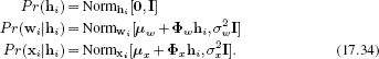
Inference in this model can be simplified by assuming that the landmark points lie exactly on the subspace so that we have the deterministic relation w_i= μ+Φh. This means that the likelihood of the observed data given the hidden variable h can be expressed as

We adopt a maximum likelihood procedure and note that this criterion is based on the normal distribution so the result is a least squares cost function:

Denoting the unknown quantities by θ = {h,Ψ}, we observe that this cost function takes the general form of f[θ] = z[θ]^T z[θ] and can hence be optimized using the Gauss-Newton method (Appendix B.2.3). We initialize the unknown quantities to some sensible values and then iteratively update these values using the relation

where J is the Jacobian matrix. The entry in the m^th row and n^th column of J consists of the derivative of the m^th element of z with respect to the n^th element of the parameter vector θ:

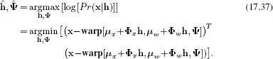
Figure 17.17 Fitting a statistical model of shape and appearance. a) Shape model at start of fitting process superimposed on the observed image. b) Shape and appearance model (synthesized image x) at start of fitting process. c-d) After several iterations. e-f) At the end of the fitting procedure. The synthesized face (f) looks very similar to the observed image in (a),(c), and (e). Such models are known as active appearance models as they can be seen to adapt to the image. Figure provided by Tim Cootes.

Figure 17.17 shows an example of a statistical shape and appearance model being fit to face data. The spine model in Figure 17.1 was also a model of this kind although only the shape component was shown. As usual, the success of this fitting procedure relies on having a good starting point for the optimization process and a course-to-fine strategy can help the optimization converge.

17.8 Non-Gaussian statistical shape models

The statistical shape model discussed in Section 17.4 is effective for objects where the shape variation is relatively constrained and is well described by the normally distributed prior. However, in some situations a normal distribution will not suffice, and we must turn to more complex models. One possibility is to use a mixture of PPCAs, and this is straightforward to implement. However, we will use this opportunity to introduce an alternative model for describing non-Gaussian densities.

The Gaussian process latent variable model or GPLVM is a density model that can model complex non-normal distributions. The GPLVM extends the PPCA model so that the hidden variables h_i are transformed through a fixed nonlinearity before being weighted by the basis functions Φ.

17.8.1 PPCA as regression

To help understand the GPLVM, we will reconsider subspace models in terms of regression. Consider the PPCA model, which can be expressed as

The first term in the last line of this expression has a close relationship to linear regression (Section 8.1); it is a model for predicting w given the variable h. Indeed if we consider just the d^th element w_d of w then this term has the form

where μ_d is the d^th dimension of μ and ^T_d• is the d^throw of Φ; this is exactly the linear regression model for w_d against h.

This insight provides a new way of looking at the model. Figure 17.18 shows a 2D data set {w_i}^I_{i = 1}, which is explained by a set of 1D hidden variables {h_i}^I_{i = 1}. Each dimension of the 2D data w is created by a different regression model, but in each case we are regressing against the common set of hidden variables {h_i}^I_{i = 1}. So, the first dimension w₁ of w is described as μ₁+^T_1•h and the second dimension w₂ is modeled as μ₂+^T_2•h. The common underlying hidden variable induces the correlation we see in the distribution Pr(w).

Now let us consider how the overall density is formed. For a fixed value of h, we get a prediction for w₁ and a prediction for w₂ each of which has additive normal noise with the same variance (Figures 17.18b-c). The result is a 2D spherical normal distribution in w. To create the density, we integrate over all possible values of h, weighted by a the normal prior; the final density is hence an infinite weighted sum of the 2D spherical normal distributions predicted by each value of h, and this happens to have the form of the normal distribution with nonspherical covariance ²+σ²I, which is seen in Figure 17.18a.

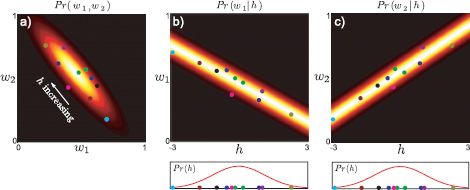
Figure 17.18 PPCA model as regression. a) We consider a 2D data set that is explained by a PPCA model with a single hidden variable. The data are explained by a 2D normal distribution with mean μ and covariance ^T+σ²I. b) One way to think of this PPCA model is that the 2D data are explained by two underlying regression models. The first data dimension w₁ is formed from a regression against h and c) the second data dimension w₂ is formed from a different regression against the same values h.

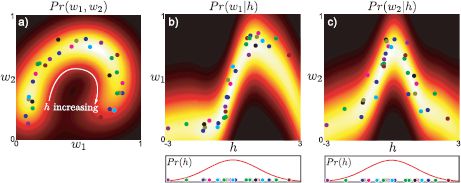
Figure 17.19 Gaussian process latent variable model as regression. a) We consider a 2D data set that is explained by a GPLVM with a single variable. b) One way to consider this model is that the 2D data are explained by two underlying regression models. The first data dimension w₁ is formed from a Gaussian process regression against the hidden variable h. c) The second data dimension w₂ is formed from a different Gaussian process regression model against the same values h.

17.8.2 Gaussian process latent variable model

This interpretation of PPCA provides an obvious approach to describing more complex densities; we simply replace the linear regression model with a more sophisticated nonlinear regression model. As the name suggests, the Gaussian process latent variable model makes use of the Gaussian process regression model (see Section 8.5).

Figure 17.19 illustrates the GPLVM. Each dimension of the density in Figure 17.19a once again results from a regression against a common underlying variable h. However, in this model, the two regression curves are nonlinear (Figures 17.19b-c) and this accounts for the complexity of the original density.

There are two major practical changes in the GPLVM:

1. In Gaussian process regression, we marginalize over the regression parameters μ and Φ so we do not have to estimate these in the learning procedure.

2. Conversely, it is no longer possible to marginalize over the hidden variables h in closed form; we must estimate the hidden variables during the training procedure. The inability to marginalize over the hidden variables also creates some difficulties in evaluating the final density.

We will now consider learning and inference in this model in turn.

Learning

In the original Gaussian process regression model (Section 8.5), we aimed to predict the univariate world states w = [w₁,w₂,…,w_I]^T from multivariate data X = [x₁,x₂,…,x_I]. The parameter vector was marginalized out of the model, and the noise parameter σ² was found by maximizing the marginal likelihood:

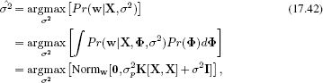
where σ²_p controls the prior variance of the parameter vector and K[•,•] is the chosen kernel function.

In the GPLVM we have a similar situation. We aim to predict multivariate world values W=[w₁,w₂,…,w_I]^T from multivariate hidden variables H=[h₁,h₂,…,h_I]. Once more, we marginalize the basis functions Φ out of the model and maximize over the noise parameters σ². However, this time, we do not know the values of the hidden variables H that we are regressing against; these must be simultaneously estimated, giving the objective function:

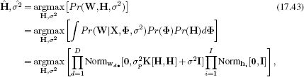
where there is one term in the first product for each of the D dimensions of the world and one term in the second product for each of the training examples.

Unfortunately, there is no closed form solution to this optimization problem; to learn the model we must use one of the general-purpose nonlinear optimization techniques discussed in Appendix B. Sometimes, the kernel K[•,•] also contains parameters, and these should be simultaneously optimized.

Inference

For a new value of the hidden variable h* the distribution over the d^th dimension of the world w*_d is given by the analogue of Equation 8.24:

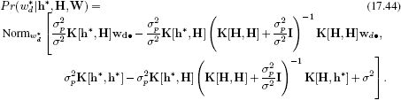
To sample from the model, we select the hidden variable h* from the prior and then predict a probability distribution over the landmarks w* using this equation.

To assess the probability of the a new sample w*, we should use the relation

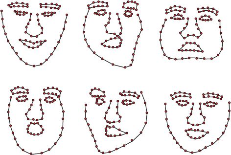
Figure 17.20 Samples from a non-Gaussian face model based on a GPLVM. The samples represent more significant distortions to the shape than could be realistically described by the original statistical shape model. Adapted from Huang et al. (2011). ©2011 IEEE.

Unfortunately, this integral cannot be computed in closed form. One possibility is to maximize over h* rather than marginalize over it. Another possibility is to approximate the density Pr(h*) by a set of delta functions at the positions of the training data {h_i})^I_i=1 and we can then replace the integral with a sum over the individual predictions from these examples.

Application to shape models

Figure 17.20 illustrates several examples of sampling from a shape model for a face that is based on the GPLVM. This more sophisticated model can cope with modeling larger variations in the shape than the original PPCA, which was based on a single normal distribution.

17.9 Articulated models

Statistical shape models work well when the shape variation is relatively small. However, there are other situations where we have much stronger a priori knowledge about the object. For example, in a body model, we know that there are two arms and two legs and that these are connected in a certain way to the main body. An articulated model parameterizes the model in terms of the joint angles and the overall transformation relating one root component to the camera.

The core idea of an articulated model is that the transformations of the parts are cumulative; the position of the foot depends on the position of the lower leg, which depends on the position of the upper leg and so on. This is known as a kinematic chain. To compute the global transformation of the foot relative to the camera, we chain the transformations relating each of the body parts in the appropriate order.

There are many approaches to constructing articulated models. They may be two dimensional (e.g., the pictorial structures discussed in Chapter 11) or exist in three dimensions. We will consider a 3D hand model that is constructed from truncated quadrics of the conic (see Section 17.1) and can represent cylinders, spheres, ellipsoids, a pair of planes, and other shapes in 3D. Points in 3D which lie on the surface of the quadric satisfy the relation

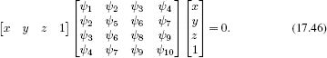
Figure 17.21 illustrates a hand model that was constructed from a set of 39 quadrics. Some of these quadrics are truncated; to make a tube shape of finite length, a cylinder or ellipsoid is clipped by a pair of planes in 3D so that only parts of the quadric that are between the planes are retained. The pair of planes is represented by a second quadric, so each part of the model is actually represented by two quadrics. This model has 27 degrees of freedom, 6 for the global hand position, 4 for the pose of each finger, and 5 for the pose of the thumb.

The quadric is a sensible choice because its projection through a pinhole camera takes the form of a conic and can be computed in closed form. Typically, an ellipsoid (represented by a quadric) would project down to an ellipse in the image (represented by a conic), and we can find a closed form expression for the parameters of this conic in terms of the quadric parameters.

Given the camera position relative to the model, it is possible to project the collection of quadrics that form the 3D model into the camera image. Self occlusion can be handled neatly by testing the depth along each ray and not rendering the resulting conic if the associated quadric lies behind another part of the model. This leads to a straightforward method for fitting the model to an image of the object (i.e., finding the joint angles and overall pose relative to the camera). We simulate a set of contours for the model (as in Figure 17.21d) and then evaluate an expression for the likelihood that increases when these match the observed edges in the image. To fit the model, we simply optimize this cost function.

Unfortunately, this algorithm is prone to converging to local minima; it is hard to find a good starting point for the optimization. Moreover, the visual data may be genuinely ambiguous in a particular image, and there may be more than one configuration of the object that is compatible with the observed image. The situation becomes more manageable if we view the object from more than one camera (as in Figures 17.21e-f and h-i) as much of the ambiguity is resolved. Fitting the model is also easier when we are tracking the model through a series of frames; we can initialize the model fitting at each time based on the known position of the hand at the previous time. This kind of temporal model is investigated in Chapter 19.

17.10 Applications

We will now look at two applications that extend the ideas of this chapter into 3D. First, we will consider a face model that is essentially a 3D version of the active appearance model. Second, we will discuss a model for the human body that combines the ideas of the articulated model and the subspace representation of shape.

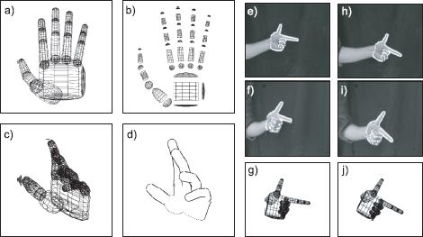
Figure 17.21 Articulated model for a human hand. a) A three-dimensional model for a human hand is constructed from 39 truncated quadrics. b) Exploded view. c) The model has 27 degrees of freedom that control the joint angles. d) It is easy to project this model into an image and find the outer and occluding contours, which can then be aligned with contours in an image. e-f) Two views of a hand taken simultaneously from different cameras g) Estimated state of hand model. h-j) Two more views and another estimate of the position. Adapted from Stenger et al. (2001a). ©2001 IEEE.

17.10.1 Three dimensional morphable models

Blanz and Vetter (1999) developed a statistical model of the 3D shape and appearance of faces. Their model was based on 200 laser scans. Each face was represented by approximately 70,000 3D vertices and an RGB texture map. The captured faces were preprocessed so that the global 3D transformation between them was removed, and the vertices were registered using a method based on optical flow.

A statistical shape model was built where the 3D vertices now take on the role of the landmark points. As with most of the statistical shape models in this chapter, this model was based on a linear combination of basis functions (principal components). Similarly, the texture maps were described as a linear combination of a set of basis images (principal components). Figure 17.22 illustrates the mean face and the effect of varying the shape and texture components independently.

The model, as described so far, is thus a 3D version of the model for shape and appearance that we described in Section 17.7. However, in addition, Blanz and Vetter (1999) model the rendering process using the Phong shading model which includes both ambient and directional lighting effects.

To fit this model to a photograph of a face, the square error between the observed pixel intensities and those predicted from the model is minimized. The goal then is to manipulate the parameters of the model so that the rendered image matches the observed image as closely as possible. These parameters include:

• The weightings of the basis functions that determine the shape,

• The weightings of the basis functions that determine the texture,

• The relative position of the camera and the object,

• The RGB intensities of the ambient and directed light, and

• The offsets and gains for each image RGB channel.

Other parameters such as the camera distance, light direction, and surface shininess were fixed by hand. In practice, the fitting was accomplished using a nonlinear optimization technique. Figure 17.23 illustrates the process of fitting the model to a real image. After convergence, the shape and texture closely replicate the original image. At the end of this process, we have full knowledge of the shape and texture of the face. This can now be viewed from different angles, relit and even have realistic shadows superimposed.

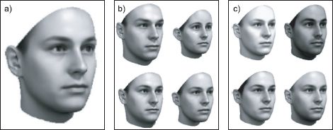
Figure 17.22 3D morphable model of a face. The model was trained from laser scans of 200 individuals and is represented as a set of 70,000 vertex positions and an associated texture map. a) Mean face. b) As for the 2D subspace shape model, the final shape is described as a linear combination of basis shapes (principal components). In this model, however, these basis shapes are three dimensional. The figure shows the effect of changing the weighting of these basis functions while keeping the texture constant. c) The texture is also modeled as a linear combination of basis shapes. The figure shows the effect of changing the texture while keeping the shape constant. Adapted from Blanz and Vetter (2003). ©2003 IEEE.

Blanz and Vetter (Blanz and Vetter 2003; Blanz et al. 2005) applied this model to face recognition. In the simplest case, they described the fitted face using a vector containing the weighting functions for both the shape and texture. Two faces can be compared by examining the distance between the vector associated with each. This method has the advantage that the faces can be originally presented in very different lighting conditions and with very different poses as neither of these factors is reflected in the final representation. However, the method is limited in practice by the model-fitting procedure, which does not always converge for real images that may suffer from complex lighting conditions and partial occlusion.

Matthews et al. (2007) presented a simplified version of the same model; this was still 3D but had a sparser mesh and did not include a reflectance model. However, they describe an algorithm for fitting this face model to video sequences that can run at more than 60 frames per second. This permits real-time tracking of the pose and expression of faces (Figure 17.24). This technique has been used to capture facial expressions for CGI characters in movies and video games.

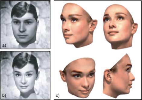
Figure 17.23 Fitting a 3D morphable model to a real image of Audrey Hepburn. The goal is to find the parameters of the 3D model that best describe the 2D face. Once we have done this, we can manipulate the image. For example we could relight the face or view it from different angles. a) Simulated image from model with initial parameters. b) Simulated image from model after fitting procedure. This closely replicates the original image in terms of both texture and shape. c) Images from fitted model generated under several different viewing conditions. Adapted from Blanz and Vetter (1999). ©1999 ACM.

17.10.2 Three-dimensional body model

Anguelov et al. (2005) presented a 3D body model that combines an articulated structure with a subspace model. The articulated model describes the skeleton of the body, and the subspace model describes the variation of the shape of the individual around this skeleton (Figure 17.25).

At its core, this model is represented by a set of triangles that define the surface of the body. The model is best explained in terms of generation in which each triangle undergoes a series of transformations. First, the position is deformed in a way that depends on the configuration of the nearest joints in the body. The deformation is determined using a regression model and creates subtle effects such as the deformation of muscles. Second, the position of the triangle is deformed according to a PCA model which determines the individuals characteristics (body shape, etc.). Finally, the triangle is warped in 3D space depending on the position of the skeleton.

Two applications of this model are shown in Figure 17.26. First, the model can be used to fill in missing parts of partial scans of human beings. Many scanners cannot capture a full 3D model at once; they may only capture the front of the object and so several scans must be combined to get a full model. This is problematic for moving objects such as human beings. Even for models that can capture 360° of shape, there are often missing or noisy parts of the data. Figure 17.26a shows an example of fitting the model to a partial scan; the position of the skeleton and the weighting of the PCA components are adapted until the synthesized shape agrees with the partial scan. The remaining part of the synthesized shape plausibly fills in the missing elements.

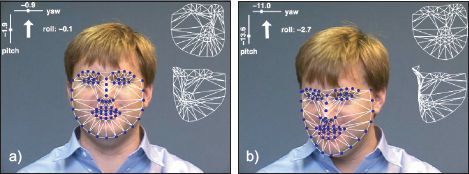
Figure 17.24 Real-time facial tracking using a 3D active appearance model. a-b) Two examples from tracking sequence. The pose of the face is indicated in the top left-hand corner. The superimposed mesh shown to the right of the face illustrates two different views of the shape component of the model. Adapted from Matthews et al. (2007). ©2007 Springer.

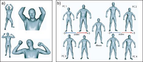
Figure 17.25 3D body model. a) The final position of the skin surface is regressed against the nearest joint angles; this produces subtle effects such as the bulging of muscles. b) The final position of the skin surface also depends on a PCA model which describes between-individual variation in body shape. Adapted from Anguelov et al. (2005). ©2005 ACM.

Figures 17.26b-d illustrate the use of the model for motion capture based animation. An actor in a motion capture studio has his body position tracked, and this body position can be used to determine the position of the skeleton of the 3D model. The regression model then adjusts the vertices of the skin model appropriately to model muscle deformation while the PCA model allows the identity of the resulting model to vary. This type of system can be used to generate character animations for video games and movies.

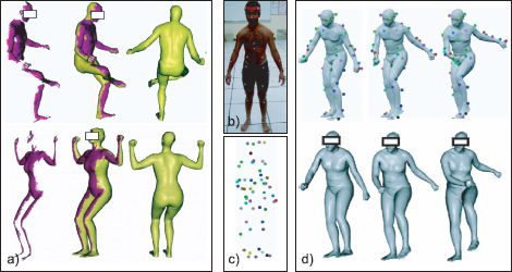
Figure 17.26 Applications of 3D body model. a) Interpolation of partial scans. In each case, the purple region represents the original scan and the green region is the interpolated part after fitting a 3D body model (viewed from two angles). b) Motion capture animation. An actor is tracked in a conventional motion capture studio. c) This results in the known position of a number of markers on the body. d) These markers are used to position the skeletal aspect of the model. The PCA part of the model can control the shape of the final body (two examples shown). Adapted from Anguelov et al. (2005). ©2005 ACM.

Discussion

In this chapter, we have presented a number of models for describing the shape of visual objects. These ideas relate closely to the subsequent chapters in this book. These shape models are often tracked in video sequences and the machinery for this tracking is developed in Chapter 19. Several of the shape models have a subspace (principal component) representation at their core. In Chapter 18 we investigate models that exploit this type of representation for identity recognition.

Notes

Snakes and active contour models: Snakes were first introduced by Kass et al. (1987). Various modifications have been made to encourage them to converge to a sensible answer including the addition of a ballooning term (Cohen 1991) and a new type of external force field called gradient vector flow (Xu and Prince 1998). The original description treated the contour as a continuous object, but subsequent work also considered it as discrete and used greedy algorithms or dynamic programming methods for optimization (Amini et al. 1990; Williams and Shah 1992). Subsequent work has investigated the use of prior information about object shape and led to active contour models (Cootes et al. 1995). This is still an open research area (e.g., Bergtholdt et al. 2005; Freifeld et al. 2010).

The contour models discussed in this chapter are known as parametric because the shape is explicitly represented. A summary of early work on parametric active contours can be found in Blake and Isard (1998). A parallel strand of research investigates implicit or nonparametric contours in which the contour is implicitly defined by the level sets of a function defined on the image domain (Malladi et al. 1994; Caselles et al. 1997). There has also been considerable interest in applying prior knowledge to these models (Leventon et al. 2000; Rousson and Paragios 2002).

Bottom-up models: This chapter has concerned top-down approaches to contour detection in which a generative model for the object is specified that explains the observed edges in the image. However, there has also been a recent surge of research progress into bottom-up approaches, in which edge fragments are combined to form coherent shapes. For example, opelt et al. (2006) introduced the “Boundary fragment model” in which pairs of edge fragments vote for the position of the centroid of the object and the object is detected by finding the position with the most support. Shotton et al. (2008a) present a similar model that incorporates scale invariance and searches through local regions of the image to identify objects that form only a small part of a larger scene. Pairwise constraints between features were introduced by Leordeanu et al. (2007). Other work has investigated reconstructing pieces of the contour as combinations of local geometric primitives such as line segments and ellipses (Chia et al. 2010).

Subspace models: The statistical models in this chapter are based on subspace models such as probabilistic PCA (Tipping 2001) although in their original presentation they used regular (non-probabilistic) PCA (see Section 13.4.2). The models could equally have been built using factor analysis (Rubin and Thayer 1982). This has the disadvantage that it cannot be learned in closed form but can cope with modeling the joint distribution of quantities that are expressed in different units (e.g., shape and texture in active appearance models). Nonlinear generalizations of PCA (Schölkopf et al. 1998) and factor analysis (Lawrence 2005) have extended these statistical models to the non-Gaussian case.

Active shape and appearance models: More details about active shape models can be found in Cootes et al. (1995). More details about active appearance models can be found in Cootes et al. (2001) and Stegmann (2002). Jones and Soatto (2005) presented an interesting extension to active appearance models in which the objects was modeled as a number of superimposed layers. Recent interest in active appearance models has focussed on improving the efficiency of fitting algorithms (Matthews and Baker 2004; Matthews et al. 2007; Amberg et al. 2009). They have been applied to many tasks including face recognition, face pose estimation and expression recognition (Lanitis et al. 1997), and lip reading (Matthews et al. 2002). Several authors have investigated nonlinear approaches including systems based on mixture models (Cootes and Taylor 1997), kernel PCA (Romdhani et al. 1999), and the GPLVM (Huang et al. 2011).

3D Morphable models: Morphable models for faces were first introduced by Blanz and Vetter (1999) and were subsequently applied to editing images and video Blanz et al. 2003), for face recognition (Blanz and Vetter 2003; Blanz et al. 2005), and for tracking 3D faces (Matthews et al. 2007). A related model has been developed for vehicles (Leotta and Mundy 2011).

Body Tracking: Generative models for tracking human bodies have been developed based on a number of representations including cylinders (Hogg 1983), ellipsoids (Bregler and Malik 1998), stick men (Mori et al. 2004), and meshes (Shakhnarovich et al. 2003). As well as 3D models, attempts have also been made to fit purely 2D models (e.g., Felzenszwalb and Huttenlocher 2005, and Rehg et al. 2003). Some research has focused on multicamera setups which help disambiguate the observed data (e.g., Gavrila and Davis 1996). Models for tracking the body in time sequences have attracted a lot of attention (e.g., Deutscher et al. 2000; Sidenbladh et al. 2000 and see Chapter 19). Recent work has attempted to leverage knowledge of the physics of the body movement to improve the results (Brubaker et al. 2010). There are also a number of approaches to body tracking based on regression (see Chapter 8). Reviews of human motion tracking can be found in Forsyth et al. (2006), Moeslund et al. (2006), Poppe (2007), and Sigal et al. (2010).

Body models for graphics: The work of Anguelov et al. (2005), who combined the skeletal and statistical shape models, was preceeded by Allen et al. (2003) and Seo and Magnenat-Thalmann (2003), who also applied PCA to skeletal models for the human body, although they do not include a component that models deformations due to muscle movement.

Hand models: Many authors have developed models for tracking hands including Rehg and Kanade (1994), (1995), Heap and Hogg (1996), Stenger et al. (2001a), Wu et al. (2001), and Lu et al. (2003). De La Gorce et al. (2008) present a very sophisticated model that describes texture, shading, and self-occlusions of the hand.

Problems

17.1 A conic is defined as the set of points where

or

Use MATLAB to draw the 2D function ^T C and identify the set of positions where this function is zero for the following matrices:

17.2 Devise an efficient algorithm to compute the distance transform. The algorithm should take a binary image and return at each pixel the city block distance to the nearest nonzero element of the original image. The city block distance d between pixels (x₁,y₁) and pixel (x₂,y₂)is defined as

17.3 Consider a prior that is based in the curvature term:

If landmark point w₁ = [100,100], and landmark point w₃ is at position w₃ = [200,300], what position w₂ will minimize the function curve [w,2]?

17.4 If the snake as described in Section 17.2 is initialized in an empty image, how would you expect it to evolve during the fitting procedure?

17.5 The spacing element of the snake prior (Equation 17.5) encourages all of the control points of the snake to be the equidistant. An alternative approach is to give the snake a tendency to shrink (so that it collapses around objects). Write out an alternative expression for the spacing term that accomplishes this goal.

17.6 Devise a method to find the “best” weight vector h given a new vector w and the parameters {μ,Φ,σ²} of the PPCA model (see Figure 17.10).

17.7 Show that if the singular value decomposition of a matrix W can be written as W = ULV^T, then it follows that

17.8 Devise a method to learn the PPCA model using the EM algorithm, giving details of both the E- and M-steps. Are you guaranteed to get the same answer as the method based on the SVD?

17.9 Show that the maximum a posteriori solution for the hidden weight variable h is as given in Equation 17.32.

17.10 You are given a set of 100 male faces and 100 female faces. By hand you mark 50 landmark points on each image. Describe how to use this data to develop a generative approach to gender classification based on shape alone. Describe both the training process and how you would infer the gender for a new face that does not contain landmark points.

17.11 Imagine that we have learned a point distribution for the shape of the human face. Now we see a new face where everything below the nose is occluded by a scarf. How could you exploit the model to estimate both the positions of the landmark points in the top half of the face and the landmark points in the (missing) bottom half of the face?

17.12 An alternative approach to building a nonlinear model of shape is to use a mixture model. Describe an approach to training a statistical shape model based on the mixture of probabilistic principal component analyzers. How would you fit this model to a new image?

17.13 One way to warp one image to another is to implement a piecewise affine warp. Assume that we have a number of points in image 1 and their corresponding points in image 2. We first triangulate each set of points in the same way. We now represent the position x₁ in image 1 as a weighted sum of the three vertices of the triangle a₁, b₁, c₁ that it lies in so that

where the weights are constrained to be positive with α+β+γ = 1. These weights are known as barycentric coordinates.

To find the position in the second image, we then compute the position relative to the three vertices a₂, b₂, c₂ of the warped triangle so that

How can we compute the weights α, β, γ? Devise a method to warp the whole image in this manner.

17.14 Consider an ellipsoid in 3D space that is represented by the quadric

where A is a 3 × 3 matrix, b is a 3 × 1 vector, and c is a scalar.

For a normalized camera we can write the world point in terms of the image point as = [^T, s]^T where s is a scaling factor that determines the distance along the ray .

(i) Combine these conditions to produce a criterion that must be true for an image point to lie within the projection of the conic.

(ii) The edge of the image of the conic is the locus of points for which there is a single solution for the distance s. Outside the conic there is no real solution for s and inside it there are two possible solutions corresponding to the front and back face of the quadric. Use this intuition to derive an expression for the conic in terms of A, b and c. If the camera has intrinsic matrix Λ, what would the new expression for the conic be?