Computer Vision: Models, Learning, and Inference (2012)

In this chapter we discuss a family of models that explain observed data in terms of several underlying causes. These causes can be divided into three types: the identity of the object, the style in which it is observed, and the remaining variation.

To motivate these models, consider face recognition. For a facial image, the identity of the face (i.e., whose face it is) obviously influences the observed data. However, the style in which the face is viewed is also important. The pose, expression, and illumination are all style elements that might be modeled. Unfortunately, many other things also contribute to the final observed data: the person may have applied cosmetics, put on glasses, grown a beard, or dyed his or her hair. These myriad contributory elements are usually too difficult to model and are hence explained with a generic noise term.

In face recognition tasks, our goal is to infer whether the identities of face images are the same or different. For example, in face verification, we aim to infer a binary variable w ∈ {0,1}, where w = 0 indicates that the identities differ and w = 1 indicates that they are the same. This task is extremely challenging when there are large changes in pose, illumination, or expression; the change in the image due to style may dwarf the change due to identity (Figure 18.1).

The models in this chapter are generative, so the focus is on building separate density models over the observed image data cases where the faces do and don’t have the same identity. They are all subspace models and describe data as a linear combination of basis vectors. We have previously encountered several models of this type, including factor analysis (Section 7.6) and PPCA (Section 17.5.1). The models in this chapter are most closely related to factor analysis, so we will start by reviewing this.

Factor analysis

Recall that the factor analysis model explained the i^th data example x_i as

where μ is the overall mean of the data. The matrix Φ = [₁, ₂,…, _K] contains K factors in its columns. Each factor can be thought of as a basis vector in a high-dimensional space, and so together they define a subspace. The Kelements of the hidden variable h_i weight the K factors to explain the observed deviations of the data from the mean. Remaining differences that cannot be explained in this way are ascribed to additive noise ∊_i which is normally distributed with diagonal covariance ∑.

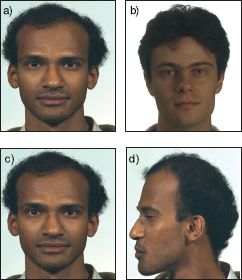
Figure 18.1 Face recognition. In face recognition the goal is to draw inferences about the identities of face images. This is difficult because the style in which the picture was taken can have a more drastic effect on the observed data than the identities themselves. For example, the images in (a-b) are more similar to one another by most measures than the images in (c-d) because the style (pose) has changed in the latter case. Nonetheless, the identities in (a-b) are different but the identities in (c-d) are the same. We must build models that tease apart the contributions of identity and style to make accurate inferences about whether the identities match.

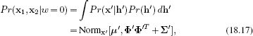
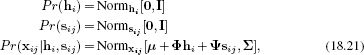
In probabilistic terms, we write

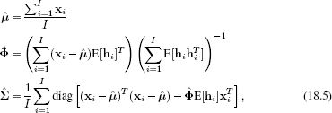
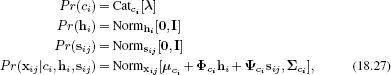
where we have also defined a suitable prior over the hidden variable h_i. Ancestral sampling from this model is illustrated in Figure 18.2.

We can compute the likelihood of observing a new data example by marginalizing over the hidden variable to get a final probability model

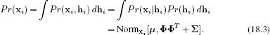
To learn this model from training data {x_i}^I_i=1, we use the expectation maximization algorithm. In the E-step, we compute the posterior distribution Pr(h_i|x_i) over each hidden variable h_i,

In the M-step we update the parameters as

where the expectations E[h_i] and E[h_ih_i^T] over the hidden variable are extracted from the posterior distribution computed in the E-step. More details about factor analysis can be found in Section 7.6.

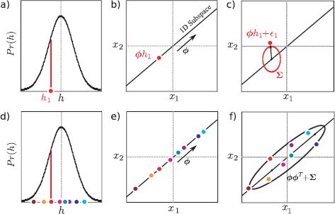
Figure 18.2 Ancestral sampling from factor analyzer. In both this figure and other subsequent figures in this chapter, we assume that the mean μ is zero. a) To generate from a factor analyzer defined over 2D data we first choose the hidden variable h_i from the normally distributed prior. Here h_i is a 1D variable and a small negative value is drawn. b) For each case we weight the factors Φ by the hidden variable. This generates a point on the subspace (here a 1D subspace indicated by black line). c) Then we add the noise term ∊_i, which is normally distributed with covariance ∑. Finally, we would add a mean term μ(not shown). d-f) This process is repeated many times. f) The final distribution of the data is a normal distribution that is oriented along the subspace. Deviations from this subspace are due to the noise term. The final covariance is ΦΦ^T + ∑.

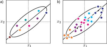
Figure 18.3 Subspace model vs. subspace identity model. a) The subspace model generates data that are roughly aligned along a subspace (here a 1D subspace defined by the black line) as illustrated in Figure 18.2. b) In the identity subspace model, the overall data distribution is the same, but there is additional structure: points that belong to the same identity (same color) are generated in the same region of space.

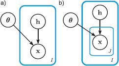
Figure 18.4 Graphical models for subspace model and subspace identity model. a) In the subspace model (factor analysis), there is one data example x_i per hidden variable h_i and some other parameters θ = {μ, Φ, ∑} that describe the subspace. b) In the subspace identity model, there are J data examples x_ijper hidden variable h_i, and all of these J examples have the same identity.

18.1 Subspace identity model

The factor analysis model provides a good description of the intensity data in frontal face images: they really do lie close to a linear subspace (see Figure 7.22). However, this description of the data does not account for identity. For images that have the same style (e.g., pose, lighting), we expect faces that have the same identity to lie in a similar part of the space (Figure 18.3), but there is no mechanism to accomplish this in the original model.

We now extend the factor analysis model to take account of data examples which are known to have the same identity and show how to exploit this to make inferences about the identity of new data examples. We adopt the notation x_ij to denote the j^th of J observed data examples from the i^th of I identities (individuals). In real-world data sets, it is unlikely that we will have exactly J examples for every individual, and the models we present do not require this, but this assumption simplifies the notation.

The generative explanation for the observed data x_ij is now

where all of the terms have the same interpretations as before. The key difference is that now all of the J data examples from the same individual are formed by taking the same linear combination h_i of the basis functions ₁… _K. However, a different noise term is added for each data example, and this explains the differences between the J face images of a given individual. We can write this in probabilistic form as

where as before we have defined a prior over the hidden variables. The graphical models for both factor analysis and the subspace identity model are illustrated in Figure 18.4. Figure 18.5 illustrates ancestral sampling from the subspace identity model; as desired this produces data points that lie close together when the identity is the same.

One way to think of this is that we have decomposed the variance in the model into two parts. The between-individual variation explains the differences between data due to different identities and the within-individual variation explains the differences between data examples due to all other factors. The data density for a single datapoint remains

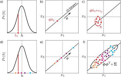
Figure 18.5 Ancestral sampling from identity subspace model. a) To generate from this model we first choose the hidden variable h_i from the normally distributed prior. Here h_i is a 1D variable and a small negative number is drawn. b) We weight the factors Φ by the hidden variable. This generates a point on the subspace. c) Then we add different noise terms {∊_ij}^J_j=1 to create each of the J examples {x_ij}^J_j=1. In each case, the noise is normally distributed with covariance ∑. Finally, we would add a mean term μ (not shown). d-f) This process is repeated several times. f) The final distribution of the data is a normal distribution with covariance ΦΦ^T +∑. However, it is structured so that points with the same hidden variable (identity) are close to one another.

However, the two components of the variance now have clear interpretations. The term ΦΦ^T corresponds to the between-individual variation, and the term ∑ is the within-individual variation.

18.1.1 Learning

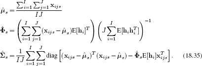
Before we consider how to use this model to draw inferences about identity in face recognition tasks, we will briefly discuss how to learn the parameters θ = {μ,Φ,∑}. As for the factor analysis model, we exploit the EM algorithm to iteratively increase a bound on the log likelihood. In the E-step we compute the posterior probability distribution over each of the hidden variables h_i given all of the data x_i• = {x_ij}^J_j=1 associated with that particular identity,

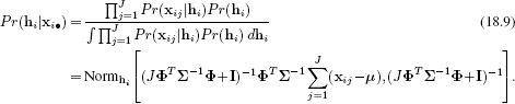
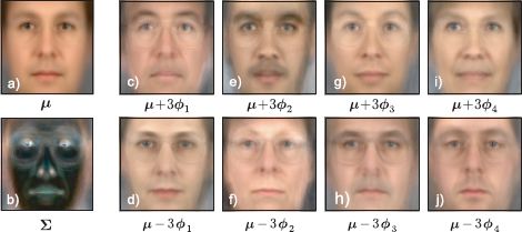
Figure 18.6 Subspace identity model parameters. These parameters were learned from J = 3 images of I = 195 individuals from the XM2VTS data set. a) Estimated mean μ. b) Estimated covariance, ∑. c-l) Four of 32 subspace directions explored by adding and subtracting multiples of each dimension to the mean.

From this we extract the moments that will be needed in the M-step,

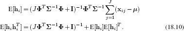
In the M-step we update the parameters using the relations

which were generated by taking the derivative of the EM bound with respect to the relevant quantities, equating the results to zero, and rearranging. We alternate the E- and M-steps until the loglikelihood of the data no longer increases.

Figure 18.6 shows parameters learned from 70 × 70 pixel face images from the XM2VTS database. A model with a K = 32 dimensional hidden space was learned with 195 identities and 3 images per person. The subspace directions capture major changes that correlate with identity. For example, ethnicity and gender are clearly represented. The noise describes whatever remains. It is most prominent around high-contrast features such as the eyes.

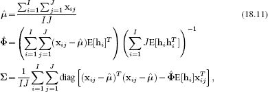
In Figure 18.7 we decompose pairs of matching images into their identity and noise components. To accomplish this, we compute the MAP hidden variable _i. The posterior over h is normal (Equation 18.9) and so the MAP estimate is simply the mean of this normal. We can then visualize the identity component μ + Φ_i, which is the same for each image of the same individual and looks like a prototypical view of that person. We can also visualize the within-individual noise = x_ij− μ − Φ_i, which explains how each image of the same person differs.

Figure 18.7 Fitting subspace identity model to new data. a−b) Original images x_i1 and x_i2. These faces can be decomposed into the sum of c−d) an identity component and e−f) a within-individual noise component. To decompose the image in this way, we computed the MAP estimate _i of the hidden variable and set the identity component to be μ + Φ_i. The noise comprises whatever cannot be explained by the identity. g−l) A second example.

18.1.2 Inference

We will now discuss how to exploit the model to make inferences about new faces that were not part of the training data set. In face verification problems, we observe two data examples x₁ and x₂ and wish to infer the state of the world w ∈ {0,1}, where w = 0 denotes the case where the data examples have different identities and w = 1 denotes the case where the data examples have the same identity.

This is a generative model, and so we calculate the posterior Pr(w|x₁, x₂) over the world state using Bayes’ rule

To compute this we need the prior probabilities Pr(w = 0) and Pr(w = 1) of the data examples having different identities or the same identity. In the absence of any other information, we might set these both to 0.5. We also need expressions for the likelihoods Pr(x₁, x₂|w = 0) and Pr(x₁, x₂|w = 1).

We will first consider the likelihood Pr(x₁, x₂|w = 0) when the two datapoints have different identities. Here, each image is explained by a different hidden variable and so the generative equation looks like

We note that this has the form of a factor analyzer:

We can reexpress this in probabilistic terms as

where ∑′ is defined as

We can now compute the likelihood Pr(x₁, x₂|w = 0) by writing the joint likelihood of the compound variables x′ and h′ and marginalizing over h′, so that

where we have used the standard factor analysis result for the integration.

For the case where the faces match (w = 1), we know that both data examples must have been created from the same hidden variable. To compute the likelihood Pr(x₁, x₂|w = 1), we write the compound generative equation

which we notice also has the form of a standard factor analyzer (Equation 18.14), and so we can compute the likelihood using the same method.

One way to think about this process is that we are comparing the likelihood for two different models of the data (Figure 18.8a). However, it should be noted that the model that categorizes the faces as different (w = 0) has two variables (h₁ and h₂), whereas the model that categorizes the faces as the same (w = 1) has only one (h₁₂). One might expect then that the model with more variables would always provide a superior explanation of the data. In fact this does not happen here, because we marginalized these variables out of the likelihoods, and so the final expressions do not include these hidden variables. This is an example of Bayesian model selection: it is valid to compare models with different numbers of parameters as long as they are marginalized out of the final solution.

18.1.3 Inference in other recognition tasks

Face verification is only one of several possible face recognition problems. Others include:

• Closed set identification: Find which one of N gallery faces matches a given probe face.

• Open set identification: Choose one of N gallery faces that matches a probe, or identify that there is no match in the gallery.

• Clustering: Given N faces, find how many different people are present and which face belongs to each person.

All of these models can be thought of in terms of model comparison (Figure 18.8). For example, consider a clustering task in which we have three faces x₁, x₂, x₃ and wish to know if (i) there are three different identities, or (ii) all of the images belong to the same person, or (iii) two images belong to the same person and the third belongs to someone different (distinguishing between the three different ways that this can happen). The world can take five states w ∈ {1,2,3,4,5} corresponding to these five situations, and each is explained by a different compound generative equation. For example, if the first two images are the same person, but the third is different we would write

which again has the form of a factor analyzer, and so we can compute the likelihood using the method described earlier. We compare the likelihood for this model to the likelihoods for the other models using Bayes’ rule with suitable priors.

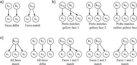
Figure 18.8 Inference as model comparison. a) Verification task. Given two faces x₁ and x₂, we must decide whether (i) they belong to different people and hence have separate hidden variables h₁, h₂ or (ii) they belong to the same person and hence share a single hidden variable h₁₂. These two hypotheses are illustrated as the two graphical models. b) Open set identification task. We are given a library {x_i}^I_i=1 of faces that belong to different people and a probe face x_p. In this case (where I = 2), we must decide whether the probe matches (i) gallery face 1, (ii) gallery face 2, or (iii) none of the gallery faces. In closed set identification, we simply omit the latter model. c) Clustering task. Given three faces x₁, x₂, and x₃, we must decide whether (i) they are all from the same person, (ii) all from different people, or (iii-v) two of the three match.

18.1.4 Limitations of identity subspace model

The subspace identity model has three main limitations (Figure 18.9).

1. The model of within-individual covariance (diagonal) is inadequate.

2. It is a linear model and cannot model non-Gaussian densities.

3. It cannot model large changes in style (e.g., frontal vs. profile faces).

We tackle these problems by introducing probabilistic linear discriminant analysis (Section 18.2), nonlinear identity models (Section 18.3), and multilinear models (Sections 18.4-18.5), respectively.

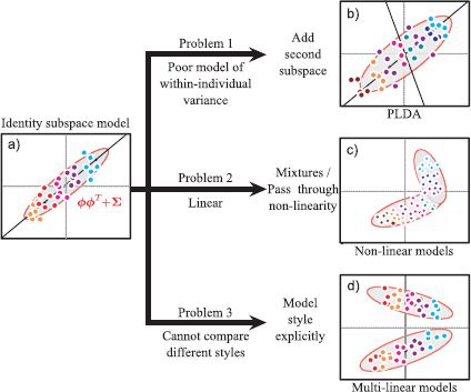
Figure 18.9 Identity models. a) There are three limitations to the subspace identity model. b) First, it has an impoverished model of the within-individual noise. To remedy this we develop probabilistic linear discriminant analysis. c) Second, it is linear and can only describe the distribution of faces as a normal distribution. Hence, we develop nonlinear models based on mixtures and kernels. d) Third, it does not work well when there are large style changes. To cope with this, we introduce multilinear models.

18.2 Probabilistic linear discriminant analysis

The subspace identity model explains the data as the sum of a component due to the identity and an additive noise term. However, the noise term is rather simple: it describes the within-individual variation as a normal distribution with diagonal covariance. The estimated noise components that we visualized in Figure 18.7 contain considerable structure, which suggests that modeling the within-individual variation at each pixel as independent is insufficient.

Probabilistic linear discriminant analysis (PLDA) uses a more sophisticated model for the within-individual variation. This model adds a new term to the generative equation that describes the within-individual variation as also lying on a subspace determined by a second factor matrix Ψ. The j^th image x_ij of the i^th individual is now described as

where s_ij is a hidden variable that represents the style of this face: it describes systematic contributions to the image from uncontrolled viewing parameters. Notice that it differs for each instance j, and so it tells us nothing about identity.

The columns of Φ describe the space of between-individual variation, and h_i determines a point in this space. The columns of Ψ describe the space of within-individual variation, and s_ij determines a point in this space. A given face is now modeled as the sum of a term μ + Φ h_i that derives from the identity of the individual, a term Ψs_ij that models the style of this particular image, and a noise term ∊_ij that explains any remaining variation (Figure 18.10).

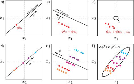
Figure 18.10 Ancestral sampling from PLDA model. a) We sample a hidden variable h_i from the identity prior and use this to weight the between-individual factors Φ. b) We sample J hidden variables {s_ij}^J_j=1 from the style prior and use these to weight the within-individual factors Ψ. c) Finally, we add normal noise with diagonal covariance, ∑. d-f) This process is repeated for several individuals. Notice that the clusters associated with each identity in (f) are now oriented (compare to Figure 18.5f); we have constructed a more sophisticated model of within-individual variation.

Once again, we can write the model in probabilistic terms:

where now we have defined priors over both hidden variables.

18.2.1 Learning

In the E-step, we collect together all the J observations {x_ij}^J_j=1 associated with the same identity to form the compound system

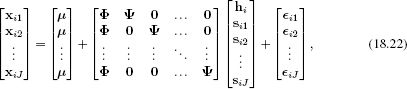
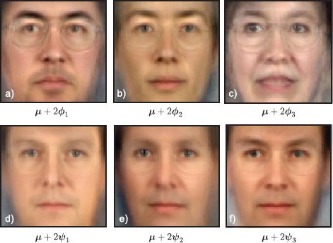
Figure 18.11 PLDA model. a-c) As we move around in the between-individual subspace Φ the images look like different people. d-f) As we move around in the within-individual subspace Ψ the images look like the same person viewed in slightly different poses and under different illuminations. The PLDA model has successfully separated out contributions that correlate with identity form those that don’t. Adapted from Li et al. (2012). ©2012 IEEE.

which takes the form of the original subspace identity model x_i′ = μ′ + Φ′h_i′ + ∊′. We can hence compute the joint posterior probability distribution over all of the hidden variables in h′ using Equation 18.9.

In the M-step we write a compound generative equation for each image,

On noting that this has the form x_ij = μ + Φ″h″_ij + ∊_ij of the standard factor analysis model, we can solve for the unknown parameters using Equations 18.5. The computations require the expectations E[h″_ij] and E[h″_ij h_ij^″T], and these can be extracted from the posterior computed in the E-step.

Figure 18.11 shows parameters learned from J = 3 examples each of I = 195 people from the XM2VTS database with 16 between-individual basis functions in Φ and 16 within-individual basis functions in Ψ. The figure demonstrates that the model has distinguished these two components.

18.2.2 Inference

As for the subspace identity model, we perform inference by comparing the likelihoods of models using Bayes’s rule. For example, in the verification task we compare models that explain the two data examples x₁ and x₂ as having either their own identities h₁ and h₂ or sharing a single identity h₁₂. When the identities are different (w = 0), the data are generated as

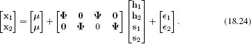
When the identities are the same (w=1), the data are generated as

Both of these formulae have the same form x′ = μ′ + Φ′h′ + ∊′ as the original factor analysis model, and so the likelihood of the data x′ after marginalizing out the hidden variables h′ is given by

where the particular choice of Φ′ comes from Equations 18.24 or 18.25, respectively. Other inference tasks concerning identity such as closed set recognition and clustering can be formulated in a similar way; we associate one value of the discrete world variable w = {1,…,K} with each possible configuration of identities, construct a generative model for each, and compare the likelihoods via Bayes’ rule.

Figure 18.12 compares closed set identification performance for several models as a function of the subspace size (for the PLDA models, the size of Ψ and Φ were always the same). The results are not state of the art: the images were not properly preprocessed, and anyway, this data set is considered relatively unchallenging. Nonetheless, the pattern of results nicely demonstrates an important point The %-correct classification improves as we increases the model’s ability to describe within-individual noise: building more complex models is worth the time and effort!

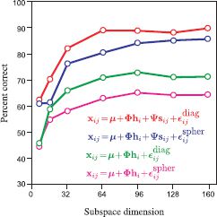
Figure 18.12 Face recognition results. The models were trained using three 70 × 70 RGB images each from 195 people from the XM2VTS database and tested using two images each from 100 different people. A gallery was formed from one image of each of the test individuals. For each of the remaining 100 test images the system had to identify the match in the gallery. Plots show %-correct performance as a function of subspace dimensionality (number of columns in Φ and ψ). Results show that as the noise model becomes more complex (adding within-individual subspace, using diagonal rather than spherical additive noise) the results improve systematically.

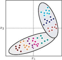
Figure 18.13 Mixture models. One way to create more complex models is to use a mixture of subspace identity models, or a mixture of PLDAs. A discrete variable is associated with each datapoint that indicates to which mixture component it belongs. If two faces belong to the same person, this must be the same; every image of the same person is associated with one mixture component. The within-individual model may also vary between components. Consequently, the within-individual variation may differ depending on the identity of the face.

18.3 Nonlinear identity models

The models discussed so far describe the between-individual and within-individual variance by means of linear models and produce final densities that are normally distributed. However, there is no particular reason to believe that the distribution of faces is normal. We now briefly discuss two methods to generalize the preceding models to the nonlinear case.

The first approach is to note that since the identity subspace model and PLDA are both valid probabilistic models, we can easily describe a more complex distribution in terms of mixtures of these elements. For example, a mixture of PLDAs model (Figure 18.13) can be written as

where c_i ∈ [1…C] is a hidden variable that determines to which of the c clusters the data belong. Each cluster has different parameters, so the full model is nonlinear. To learn this model, we embed the existing learning algorithm inside a second EM loop that associates each identity with a cluster. In inference, we assume that faces must belong to the same cluster if they match.

A second approach is based on the Gaussian process latent variable model (see Section 18.8). The idea is to induce a complex density by passing the hidden variable through a nonlinear function f[•] before using the result to weight the basis functions. For example, the generalization of the subspace identity model to the nonlinear case can be written as

Although this model is conceptually simple, it is harder to work with in practice: it is no longer possible to marginalize over the hidden variables. However, the model is still linear with respect to the factor matrix Φ, and it is possible to marginalize over this and the mean μ, giving a likelihood term of the form

This model can be expressed in terms of inner products of the transformed hidden variables f[h] and so is amenable to kernelization. Unfortunately, because we cannot marginalize over h_i, it is no longer possible exactly to compare model likelihoods directly in the inference stage. However, in practice there are ways to approximate this process.

18.4 Asymmetric bilinear models

The models that we have discussed so far are sufficient if the within-individual variation is small. However, there are other situations where the style of the data may change considerably. For example, consider the problem of face recognition when some of the faces are frontal and others profile. Unfortunately, any given frontal face has more in common visually with other non-matching frontal faces than it does with a matching profile face.

Motivated by this problem, we now develop the asymmetric bilinear model for modeling identity and style: as before, we treat the identity h_i as continuous, but now we treat the style ∈ {1…S} as discrete taking one of S possible values. For example, in the cross-pose face recognition example, = 0 might indicate a frontal face, and = 1 might indicate a profile face. The model is hence asymmetric as it treats identity and style differently. The expression of the identity depends on the style category so that the same identity may produce completely different data in different styles.

We adopt the notation x_ijs to denote the j^th of J examples of the i^th of I identities in the ^th of S styles. The data are generated as

where μ_s is a mean vector associated with the ^th style, Φ_s contains basis functions associated with the ^th style, and ∊_ijs is additive normal noise with a covariance ∑ that also depends on the style. When the noise covariances are spherical, this model is a probabilistic form of canonical correlation analysis. When the noise is diagonal, it is known as tied factor analysis. We will use the generic term asymmetric bilinear model to cover both situations.

Equation 18.30 is easy to parse; for a given individual, the identity h_i is constant. The data are explained as a weighted linear sum of basis functions, where the weights determine the identity. However, the basis functions (and other aspects of the model) are now contingent on the style.

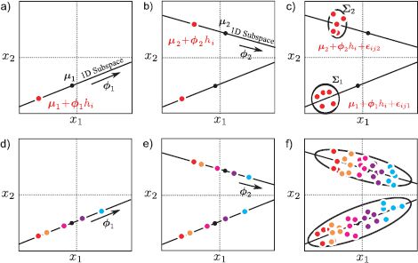
Figure 18.14 Asymmetric bilinear model with two styles. a) We draw a hidden variable h_i from the prior and use this to weight basis functions Φ₁ (one basis function ₁ shown). The result is added to the mean μ₁. b) We use the same value of h_i to weight a second set of basis functions Φ₂ and add the result to μ₂. c) We add normally distributed noise with a diagonal covariance ∑_s that depends on the style. d-f) When we repeat this procedure, it produces one normal distribution per style. The data within each style are structured so that nearby points have the same identity (color) and identities that are close in one cluster are also close in the other cluster.

We can write the model in probabilistic terms as

where λ contains parameters that determine the probability of observing data in each style. Figure 18.14 demonstrates ancestral sampling from this model. If we marginalize over the identity parameter h and the style parameter , the overall data distribution (without regard to the structure of the style clusters) is a mixture of factor analyzers,

18.4.1 Learning

For simplicity, we will assume that the styles of each training example are known and so it is also trivial to estimate the categorical parameters λ. As for the previous models in this chapter, we employ the EM algorithm.

In the E-step, we compute a posterior distribution over the hidden variable h_i that represents the identity, using all of the training data for that individual regardless of the style. Employing Bayes’ rule, we have

where x_i•• = {x_ijs}^J,S_j,=1 denotes all the data associated with the i^th individual.

One way to compute this is to write a compound generative equation for x_i••. For example, with J = 2 images at each of S = 2 styles we would have

which has the same form as the identity subspace model, x′_ij = μ′ + Φ′h_i + ∊′_ij. We can hence compute the posterior distribution using Equation 18.9 and extract the expected values needed for the M-step using Equation 18.10.

In the M-step we update the parameters θ_s = {μ_s, Φ, ∑} for each style separately using all of the relevant data. This gives the updates

As usual, we iterate these two steps until the system converges and the log likelihood ceases to improve. Figure 18.15 shows examples of the learned parameters for a data set that includes faces at two poses.

18.4.2 Inference

There are a number of possible forms of inference in this model. These include:

1. Given x, infer the style ∈ {1,…,S}.

2. Given x, infer the parameterized identity h.

3. Given x₁ and x₂, infer whether they have the same identity or not.

4. Given x₁ in style ₁, translate the style to ₂ to create ₂.

We will consider each in turn.

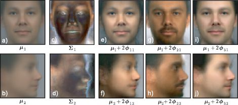
Figure 18.15 Learned parameters of asymmetric bilinear model with two styles (frontal and profile faces). This model was learned from one 70 × 70 image of each style in 200 individuals from the FERET data set. a-b) Mean vector for each style. c-d) Diagonal covariance for each style. e-f) Varying first basis function in each style (notation _ks denotes k^th basis function of ^th style). g-h) Varying second basis function in each style. i-l) Varying third basis function in each style. Manipulating the two sets of basis functions in the same way produces images that look like the same person, viewed in each of the styles. Adapted from Prince et al. (2008). ©2008 IEEE.

Inferring style

The likelihood of the data given style but regardless of identity h is

The posterior Pr(|x) over style can be computed by combining this likelihood with the prior Pr() using Bayes’ rule. The prior for style s is given by

Inferring identity

The likelihood of the data given style h but regardless of style is

The posterior over identity can now be combined with the prior Pr(h) using Bayes' rule and is given by

Note that this posterior distribution is a mixture of Gaussians, with one component for each possible style.

Identity matching

Given two examples x₁, x₂, compute the posterior probability that they have the same identity, even though they may be viewed in different styles. We will initially assume the styles are known and are ₁ and ₂, respectively. We first build the compound model

which represents the case where the identities differ (w = 0). We compute the likelihood by noting that this has the form x′ = μ′ + Φ′h′ + ∊′ of the original factor analyzer, and so we can write

where ∑′ is a diagonal matrix containing the (diagonal) covariances of the elements of ∊′ (as in Equation 18.16).

Similarly, we can build a system for when the identities match (w = 1)

and compute its likelihood Pr(x′|w = 1) in the same way. The posterior probability Pr(w = 1|x′) can then be computed using Bayes’ rule.

If we do not know the styles, then each likelihood term will become a mixture of Gaussians where each component has the form of Equation 18.41. There will be one component for every one of the S² combinations of the two styles. The mixing weights will be given by the probability of observing that combination so that Pr(₁ = m, ₂ = n) = λ_m λ._n.

Style translation

Finally, let us consider style translation. Given observed data x in style ₁ translate to the style ₂ while maintaining the same identity. A simple way to get a point estimate of the translated styles is to first estimate the identity variable h based on the observed image x₁. To do this, we compute the posterior distribution over the hidden variable

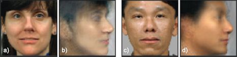
Figure 18.16 Style translation based on asymmetric bilinear model from Figure 18.15. a) Original face in style 1 (frontal). b) Translated to style 2 (profile). c-d) A second example. Adapted from Prince et al. (2008). ©2008 IEEE.

and then set h to the MAP estimate

which is just the mean of this distribution.

We then generate the image in the second style as

which is the original generative equation with the noise term omitted.

18.5 Symmetric bilinear and multilinear models

As the name suggests, symmetric bilinear models treat both style and identity equivalently. Both are continuous variables, and the model is linear in each. To write these models in a compact way, it is necessary to introduce tensor product notation. In this notation (see Appendix C.3), the generative equation for the subspace identity model (Equation 18.6) is written as

where the notation Φ × ₂ h_i means take the dot product of the second dimension of Φ with h_i. Since Φ was originally a 2D matrix, this returns a vector.

In the symmetric bilinear model, the generative equation for the j^th example of the i^th identity in the k^th style is given by

where h_i is a 1D vector representing the identity, s_k is a 1D vector representing the style, and Φ is now a 3D tensor. In the expression Φ ×₂ h_i ×₃s_k we take the dot product with two of these three dimensions, leaving a column vector as desired.

In probabilistic form, we write

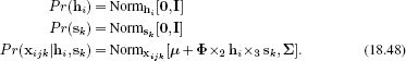
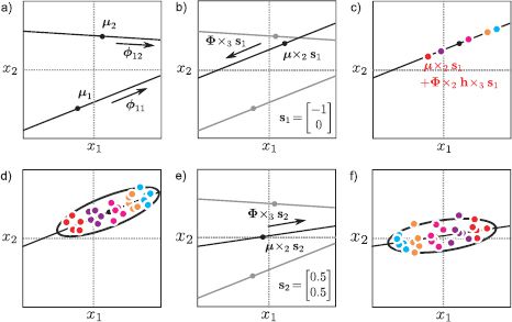
Figure 18.17 Ancestral sampling from symmetric bilinear model, with 1D identity and 2D style. a) In this model each style dimension consists of a subspace identity model with a 1D subspace. b) For a given style vector s₁, we weight these models to create a new subspace identity model. c) We then generate from this by weighting the factor by the hidden variable h and d) adding noise to generate different instances of this identity in this style. e) A different weighting induced by the style vector s₂ creates a different subspace model. f) Generation from the resulting subspace identity model.

For a fixed style vector s_k this model is exactly a subspace identity model with hidden variable h_i The choice of style determines the factors by weighting a set of basis functions to create them. It is also possible to make the mean vector depend on the style by using the model

where μ is now a matrix with basis functions in the columns that are weighted by the style . Ancestral sampling from this model is illustrated in Figure 18.17.

It is instructive to compare the asymmetric and symmetric bilinear models. In the asymmetric bilinear model, there were a discrete number of styles each of which generated data that individually looked like a subspace identity model, but the model induced a relationship between the position of an identity in one style cluster and in another. In the symmetric bilinear model, there is a continuous family of styles that produces a continuous family of subspace identity models. Again the model induces a relationship between the position of an identity in each.

Up to this point, we have described the model as a subspace identity model for fixed style. The model is symmetric, and so it is possible to reverse the roles of the variables. For a fixed identity, the model looks like a subspace model where the basis functions are weighted by the variable s_k. In other words, the model is linear in both sets of hidden variables when the other is fixed. It is not, however, simultaneously linear in both h and s together. These variables have a nonlinear interaction, and overall the model is nonlinear.

18.5.1 Learning

Unfortunately, is not possible to compute the likelihood of the bilinear model in closed form; we cannot simultaneously marginalize over both sets of hidden variables and compute

where θ = {μ, Φ, ∑} represents all of the unknown parameters. The usual approach for learning models with hidden variables is to use the EM algorithm, but this is no longer suitable because we cannot compute the joint posterior distribution over the hidden variables Pr(h_i, s_k|{x_ijk}^J_j=1) in closed form either.

For the special case of spherical additive noise ∑ = σ²I, and complete data (where we see J examples of each of the I individuals in each of K styles), it is possible to solve for the parameters in closed form using a method similar to that used for PPCA (Section 17.5.1). This technique relies on the N-mode singular value decomposition, which is the generalization of the SVD to higher dimensions.

For models with diagonal noise, we can approximate by maximizing over one of the hidden variables rather than marginalizing over them. For example, if we maximize over the style parameters so that

then the remaining model is linear in the hidden variables h_i. It would hence be possible to apply an alternating approach in which we first fix the styles and learn the parameters with the EM algorithm and then fix the parameters and update the style parameters using optimization.

18.5.2 Inference

Various forms of inference are possible, including all of those discussed for the asymmetric bilinear model. We can, for example, make decisions about whether identities match by comparing different compound models. It is not possible to marginalize over both the identity and style variables in these models, and so we maximize over the style variable in a similar manner to the learning procedure. Similarly, we can translate from one style to another by estimating the identity variable h (and the current style variable s if unknown) from the observed data. We then use the generative equation with a different style vector to simulate a new example in a different style.

The symmetric bilinear model has a continuous parameterization of style, and so it is also possible to perform a new translation task: given an example whose identity we have not previously seen and whose style we have not previously seen, we can translate either its style or identity as required. We first compute the current identity and style which can be done using a nonlinear optimization approach,

Then we simulate new examples using the generative equation, modifying the style s or identity h as required. An example of this is shown in Figure 18.18.

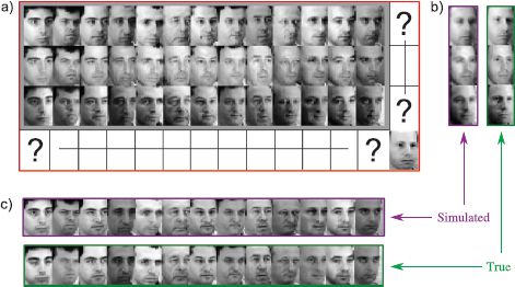
Figure 18.18 Translation of styles using symmetric bilinear model. a) We learn the model from a set of images, where the styles (rows) and identities (columns) are known. Then we are given a new image which has a previously unseen identity and style. b) The symmetric bilinear model can estimate the identity parameters and simulate the image in new styles, or c) estimate the style parameters and simulate new identities. In both cases, the simulated results are close to the ground truth. Adapted from Tenebaum and Freeman (200). ©2000 MIT Press.

18.5.3 Multilinear models

The symmetric bilinear model can be extended to create multilinear or multifactor models. For example, we might describe our data as depending on three hidden variables, h, s and t, so the generative equation becomes

and now the tensor Φ becomes four-dimensional. As in the symmetric bilinear model, it is not possible to marginalize over all of the hidden variables in closed form, and this constrains the possible methods for learning and inference.

18.6 Applications

We have illustrated many of the models in this chapter with examples from face recognition. In this section, we will describe face recognition in more detail and talk about some of the practicalities of building a recognition system. Subsequently, we will discuss an application in which a visual texture is compactly represented as a multilinear model. Finally, we will describe a nonlinear version of the multilinear model that can be used to synthesize animation data.

18.6.1 Face recognition

To provide a more concrete idea of how well these algorithms work in practice, we will discuss a recent application in detail. Li et al. (2012) present a recognition system based on probabilistic linear discriminant analysis.

Eight keypoints on each face were identified, and the images were registered using a piecewise affine warp. The final image size was 400 × 400. Feature vectors were extracted from the area of the image around each keypoint. The feature vectors consisted of image gradients at 8 orientations and three scales at points in a 6 × 6 grid centered on the keypoint. A separate recognition model was built for each keypoint and these were treated as independent in the final recognition decision.

The system was trained using only the first 195 individuals from the XM2VTS database and signal and noise subspaces of size 64. In testing, the algorithm was presented with 80 images taken from the remaining 100 individuals in the database and was required to cluster them into groups according to identity. There may be 80 images of the same person or 80 images of different people or any permutation between these extremes.

In principle it is possible to calculate the likelihood for each possible clustering of the data. Unfortunately, in practice there are far too many possible configurations. Hence, Li et al. (2012) adopted a greedy agglomerative strategy. They started with the hypothesis that there are 80 different individuals. They considered merging all pairs of individuals and chose the combination that increased the likelihood the most. They repeated this process until the likelihood could not be improved. Example clustering results are illustrated in Figure 18.19 and are typical of state-of-the-art recognition algorithms; they cope relatively easily with frontal faces under controlled lighting conditions.

However, for more natural images the same algorithms struggle even with more sophisticated preprocessing. For example, Li et al. (2012) applied the PLDA model to face verification in the “Labeled Faces in the Wild” dataset (Huang et al. 2007b), which contains images of famous people collected from the Internet, and obtained an equal-error rate of approximately 10 percent. This is typical of the state of the art at the time of writing and is much worse than for faces captured under controlled conditions.

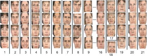
Figure 18.19 Face clustering results from Li et al. (2012). The algorithm was presented with a set of 80 faces consisting of with 4 pictures each of 20 people and clustered these almost perfectly; it correctly found 19 of these 20 groups of images but erroneously divided the data from one individual into two separate clusters. The algorithm works well for these frontal faces despite changes in expression (e.g., cluster 3), changes in hairstyle (e.g., cluster 9) and the addition or removal of glasses (e.g., cluster 4). Adapted from Li et al. (2012). ©2012 IEEE.

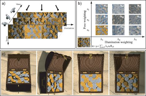
Figure 18.20 Tensor textures. a) The training set consists of renderings of a set of coins viewed from several different directions and with several different lighting directions. b) A new texture (bottom-left corner) is computed as a weighted sum of the learned basis functions stored in the 3D tensor Φ. c) Several frames of a video sequence in which the texture is synthesized appropriately from the model. Adapted from Vasilescu and Tezopoulos (2004). ©2003 ACM.

18.6.2 Modeling texture

The interaction of light with a surface can be described by the bi-directional reflectance distribution function; essentially, this describes the outgoing light at each angle from the surface given incoming light at a particular angle to the surface. The bi-directional texture function (BTF) generalizes this model to also depend on the 2D position on the surface of the object. If we know the BTF, then we know how a textured surface will appear from every angle and under every lighting combination.

This function could be approximated by taking several thousand images of the surface viewed from different angles and under different lighting conditions. However, the resulting data are clearly highly redundant. Vasilescu and Terzopoulos (2004) described the BTF using a multilinear model known as “TensorTextures.” It contained style factors that represent the lighting and viewing directions (Figure 18.20a-b). Although both of these quantities are naturally 2D, they represented them as vectors of size 21 and 37, respectively, where each training example was transformed to one coordinate axis.

Figure 18.20c shows images generated from the TensorTextures model; the hidden variables associated in each style were chosen by linearly interpolating between the hidden variables of nearby training examples, and the image was synthesized without the addition of noise. It can be seen that the TensorTextures model has learned a compact representation of the appearance variation under changes in viewpoint and illumination, including complex effects due to self-occlusion, inter-reflection, and self-shadowing.

18.6.3 Animation synthesis

Wang et al. (2007) developed a multifactor model that depended nonlinearly on the identity and style components. Their approach was based on the Gaussian process latent variable model; the style and identity factors were transformed through nonlinear functions before weighting the tensor Φ. In this type of model, the likelihood might be given by

where f[•] and g[•] are nonlinear functions that transform the identity and style parameters, respectively. In practice, the tensor Φ can be marginalized out of the final likelihood computation in closed form along with the overall mean μ. This model can be expressed in terms of inner products of the identity and style parameters and can hence be kernelized. It is known as the multifactor Gaussian process latent variable model or the multifactor GPLVM.

Wang et al. (2007) used this model to describe human locomotion. A single pose was described as an 89-dimensional vector, which consisted of 43 joint angles, the corresponding 43 angular velocities and the global translational velocity. They built a model consisting of three factors; the identity of the individual, the gait of locomotion (walk, stride, or run), and the current state in the motion sequence. Each was represented as a 3D vector. They learned the model from human capture data using an RBF kernel.

Figure 18.21 shows the results of style translation in this model. The system can predict realistic body poses in styles that have not been observed in the training data. Since the system is generative, it can also be used to synthesize novel motion sequences for a given individual in which the gait varies over time.

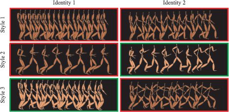
Figure 18.21 Multifactor GPLVM applied to animation synthesis. A three-factor model was learned with factors for identity, style, and position in the gait sequence. The figures shows training data (red boxes) and synthesized data from the learned model (green boxes). In each case, it manages to simulate the style and identity well. Adapted from Wang et al. (2007).

Discussion

In this chapter, we have examined a number of models that describe image data as a function of style and content variables. During training, these variables are forced to take the same value for examples where we know the style or content are the same. We have demonstrated a number of different forms of inference including identity recognition and style translation.

Notes

Face recognition: For a readable introduction to face recognition consult Chellappa et al. (2010). For more details, consult the review paper by Zhao et al. (2003) or the edited book by Li and Jain (2005).

Subspace methods for face recognition: Turk and Pentland (2001) developed the eigenfaces method in which the pixel data were reduced in dimension by linearly projecting it onto a subspace corresponding to the principal components of the training data. The decision about whether two faces matched or not was based on the distance between these low-dimensional representations. This approach quickly supplanted earlier techniques that had been based on measuring the relative distance between facial features (Brunelli and Poggio 1993).

The subsequent history of face recognition has been dominated by other subspace methods. Researchers have variously investigated the choice of basis functions (e.g., Bartlett et al. 1998; Belhumeur et al. 1997; He et al. 2005; Cai et al. 2007), analogous nonlinear techniques (Yang 2002), and the choice of distance metric (Perlibakas 2004). The relationship between different subspace models is discussed in (Wang and Tang 2004b). A review of subspace methods (without particular reference to face recognition) can be found in De La Torre (2011).

Linear discriminant analysis A notable subcategory of these subspace methods consists of approaches based on linear discriminant analysis (LDA). The Fisherfaces algorithm (Belhumeur et al. 1997) projected face data to a space where the ratio of between-individual variation to within-individual variation was maximized. Fisherfaces is limited to directions in which at least some within-individual variance has been observed (the small-sample problem). The null-space LDA approach (Chen et al. 2000) exploited the signal in the remaining subspace. The Dual-Space LDA approach (Wang and Tang 2004a) combined these two sources of information.

Probabilistic approaches: The identity models in this chapter are probabilistic reinterpretations of earlier non-probabilistic techniques. For example, the subspace identity model is very similar to the eigenfaces algorithm (Turk and Pentland 2001), and probabilistic LDA is very similar to the Fisherfaces algorithm (Belhumeur et al. 1997). For more details about these probabilistic versions, consult Li et al. (2012) and Ioffe (2006), who presented a slightly different probabilistic LDA algorithm. There have also been many other probabilistic approaches to face recognition (Liu and Wechsler 1998; Moghaddam et al. 2000; Wang and Tang 2003; Zhou and Chellappa 2004).

Alignment and pose changes: An important part of most face recognition pipelines is to accurately identify facial features so that either (i) the face image can be aligned to a fixed template or (ii) the separate parts of the face can be treated independently (Wiskott et al. 1997; Moghaddam and Pentland 1997). Common methods to identify facial features include the use of active shape models (Edwards et al. 1998) or pictorial structures (Everingham et al. 2006; Li et al. 2010).

For larger pose changes, it may not be possible to warp the face accurately to a common template, and explicit methods are required to compare the faces. These include fitting 3D morphable models to the images and then simulating a frontal image from a non-frontal one (Blanz et al. 2005), predicting the face at one pose from another using statistical methods (Gross et al. 2002; Lucey and Chen 2006) or using the tied factor analysis model discussed in this chapter (Prince et al. 2008). A review of face recognition across large pose changes can be found in Zhang and Gao (2009).

Current work in face recognition: It is now considered that face recognition for frontal faces in constant lighting and with no pose or expression changes is almost solved. Earlier databases that have these characteristics (e.g., Messer et al. 1999; Phillips et al. 2000) have now been supplanted by test databases containing more variation (Huang et al. 2007b).

Several recent trends have emerged in face recognition. These include a resurgence of interest in discriminative models (e.g., Wolf et al. 2009; Taigman et al. 2009; Kumar et al. 2009), the application of learning of metrics to discriminate identity (e.g., Nowak and Jurie 2007; Ferencz et al. 2008; Guillaumin et al. 2009; Nguyen and Bai 2010), the use of sparse representations (e.g., Wright et al. 2009), and a strong interest in preprocessing techniques. In particular, many current methods are based on Gabor features (e.g., Wang and Tang 2003), local binary patterns (Ojala et al. 2002; Ahonen et al. 2004), three-patch local binary patterns (Wolf et al. 2009), or SIFT features (Lowe 2004). Some of the most successful methods combine or select several different preprocessing techniques (Li et al. 2012; Taigman et al. 2009; Pinto and Cox 2011).

Bilinear and multilinear models: Bilinear models were introduced to computer vision by Tenenbaum and Freeman (2000), and multilinear models were explored by Vasilescu and Terzopoulos (2002). Kernelized multilinear models were discussed by Li et al. (2005) and Wang et al. (2007). An alternative approach to nonlinear multifactor models was presnented in Elgammal and Lee (2004). The most common use of bilinear and multilinear models in computer vision has been for face recognition in situations where the capture conditions vary (Grimes et al. 2003; Lee et al. 2005; Cuzzolin 2006; Prince et al. 2008).

Problems

18.1 Prove that the posterior distribution over the hidden variable in the subspace identity model is as given in Equation 18.9.

18.2 Show that the M-step updates for the subspace identity model are as given in Equation 18.11.

18.3 Develop a closed form solution for learning the parameters {μ,Φ,σ²} of a subspace identity model where the noise is spherical:

Hint: Assume you have exactly J = 2 examples of each of the I training images and base your solution on probabilistic PCA.

18.4 In a face clustering problem, how many possible models of the data are there with 2, 3, 4, 10, and 100 faces?

18.5 An alternative approach to face verification using the identity subspace model is to compute the probability of the observed data x₁ and x₂ under the models:

Write down expressions for the marginal probability terms Pr(x₁), Pr(x₂) and the conditional probability Pr(x₂|x₁). How could you use these expressions to compute the posterior Pr(w|x₁, x₂) over the world state?

18.6 Propose a version of the subspace identity model that is robust to outliers in the training data.

18.7 Moghaddam et al. (2000) took a different probabilistic approach to face verification. They took the difference x_Δ = x₂ - x₁ and modeled the likelihoods of this vector Pr(x_Δ|w = 0) and Pr(xΔ|w = 1) when the two faces match or don’t. Propose expressions for these likelihoods and discuss learning and inference in this model. Identify one possible disadvantage of this model.

18.8 Develop a model that combines the advantages of PLDA and the asymmetric bilinear model; it should be able to model the within-individual covariance with a subspace but also be able to compare data between disparate styles. Discuss learning and inference in your model.

18.9 In the asymmetric bilinear model, how would you infer whether the style of two examples is the same or not, regardless of whether the images matched?