Running Linux, 5th Edition (2009)

Part I. Enjoying and Being Productive on Linux

Chapter 9. Multimedia

This chapter is about multimedia on Linux. Multimedia is a rather vague and much abused term. For the purposes of this chapter, our loose definition is anything related to sound, graphics, or video.

Multimedia has historically been one of the more challenging areas of Linux, both for developers and users, and one that did not receive as much attention from Linux distributions as it should have, perhaps because Linux was initially embraced by so many as a server operating system. It was only recently that Linux has been seriously considered as a desktop solution for mainstream users. To be successful at attracting users from other popular operating systems, multimedia support is a requirement.

The good news is that, unlike a few years ago, most modern Linux distributions automatically detect and configure multimedia hardware for the user and provide a basic set of applications. And despite its historic use as a server, for a number of reasons Linux is well suited to audio and other multimedia applications.

We start off this chapter with a quick overview of multimedia concepts such as digital audio and video, and a description of the different types of multimedia hardware devices. Those familiar with the technology may wish to skip over this section. If you don't really care about how it all works or get lost in the first sentence of this section, don't worry, you can get applications up and running without understanding the difference between an MP3 and a WAV file. The section "Movies and Music: Totem and Rhythmbox" in Chapter 3 describes the basic playback tools offered on most Linux desktops.

We then discuss some of the issues related to multimedia support at the kernel level, which is a prerequisite for using the hardware. We then move on to applications, first those offered by some of the popular desktop environments, and then a sampling of more specialized applications broken down into different categories. If you want to develop your own applications, we briefly cover some of the popular toolkits and development environments. Finally, we wrap things up with a list of references in print and on the Web where you can find information that is more detailed and current.

Keep in mind that multimedia is an area where Linux development moves rapidly and new technologies quickly move from primitive prototypes to mainstream usage. In 1996, in a book on multimedia on Linux, we wrote about a technology called MPEG-1 layer 3, or MP3. At the time it was relatively unknown, used only by some obscure web sites to distribute music, and my then-current 40 MHz Intel 386 computer was barely able to decode it in real time. Not so many years later, it has become ubiquitous and the de facto standard file format for digital music on the Internet. At the same time, other technologies that appeared promising have fallen by the wayside, often not for technical reasons. To stay current, check the resources listed at the end of the chapter.

There are minor differences among Linux distributions. Although most of the information in this chapter is generic and applicable to most Linux distributions, for details you should consult the documentation that came with your system, contact your distribution vendor, or consult with fellow users.

Multimedia Concepts

This section very quickly covers some concepts relevant to digital audio , video , and sound cards . Understanding these basics will help you follow the rest of the material in this chapter.

Digital Sampling

Sound is produced when waves of varying pressure travel though a medium, usually air. It is inherently an analog phenomenon, meaning that the changes in air pressure can vary continuously over a range of values.

Modern computers are digital, meaning they operate on discrete values, essentially the binary ones and zeroes that are manipulated by the central processing unit (CPU). In order for a computer to manipulate sound, then, it needs to convert the analog sound information into digital format.

A hardware device called an analog-to-digital converter converts analog signals, such as the continuously varying electrical signals from a microphone, to digital format that can be manipulated by a computer. Similarly, a digital-to-analog converter converts digital values into analog form so they can be sent to an analog output device such as a speaker. Sound cards typically contain several analog-to-digital and digital-to-analog converters .

The process of converting analog signals to digital form consists of taking measurements, or samples, of the values at regular periods of time, and storing these samples as numbers. The process of analog-to-digital conversion is not perfect, however, and introduces some loss or distortion. Two important factors that affect how accurately the analog signal is represented in digital form are the sample size and sampling rate.

The sample size is the range of values of numbers that is used to represent the digital samples, usually expressed in bits. For example, an 8-bit sample converts the analog sound values into one of 2⁸, or 256, discrete values. A 16-bit sample size represents the sound using 2¹⁶, or 65,536, different values. A larger sample size allows the sound to be represented more accurately, reducing the sampling error that occurs when the analog signal is represented as discrete values. The trade-off with using a larger sample size is that the samples require more storage (and the hardware is typically more complex and therefore expensive).

The sample rate is the speed at which the analog signals are periodically measured over time. It is properly expressed as samples per second, although sometimes informally but less accurately expressed in Hertz (Hz) . A lower sample rate will lose more information about the original analog signal, a higher sample rate will more accurately represent it. The sampling theorem states that to accurately represent an analog signal it must be sampled at at least twice the rate of the highest frequency present in the original signal.

The range of human hearing is from approximately 20 to 20,000 Hz under ideal situations. To accurately represent sound for human listening, then, a sample rate of twice 20,000 Hz should be adequate. CD player technology uses 44,100 samples per second, which is in agreement with this simple calculation. Human speech has little information above 4000 Hz. Digital telephone systems typically use a sample rate of 8000 samples per second, which is perfectly adequate for conveying speech. The trade-off involved with using different sample rates is the additional storage requirement and more complex hardware needed as the sample rate increases.

Other issues that arise when storing sound in digital format are the number of channels and the encoding format. To support stereo sound, two channels are required. Some audio systems use four or more channels.

Often sounds need to be combined or changed in volume. This is the process of mixing, and can be done in analog form (e.g., a volume control) or in digital form by the computer. Conceptually, two digital samples can be mixed together simply by adding them, and volume can be changed by multiplying by a constant value.

Up to now we've discussed storing audio as digital samples. Other techniques are also commonly used. FM synthesis is an older technique that produces sound using hardware that manipulates different waveforms such as sine and triangle waves. The hardware to do this is quite simple and was popular with the first generation of computer sound cards for generating music. Many sound cards still support FM synthesis for backward compatibility. Some newer cards use a technique called wavetable synthesis that improves on FM synthesis by generating the sounds using digital samples stored in the sound card itself.

MIDI stands for Musical Instrument Digital Interface. It is a standard protocol for allowing electronic musical instruments to communicate. Typical MIDI devices are music keyboards, synthesizers, and drum machines. MIDI works with events representing such things as a key on a music keyboard being pressed, rather than storing actual sound samples. MIDI events can be stored in a MIDI file, providing a way to represent a song in a very compact format. MIDI is most popular with professional musicians, although many consumer sound cards support the MIDI bus interface.

File Formats

We've talked about sound samples, which typically come from a sound card and are stored in a computer's memory. To store them permanently, they need to be represented as files. There are various methods for doing this.

The most straightforward method is to store the samples directly as bytes in a file, often referred to as raw sound files. The samples themselves can be encoded in different formats. We've already mentioned sample size, with 8-bit and 16-bit samples being the most common. For a given sample size, they might be encoded using signed or unsigned representation. When the storage takes more than 1 byte, the ordering convention must be specified. These issues are important when transferring digital audio between programs or computers, to ensure they agree on a common format.

A problem with raw sound files is that the file itself does not indicate the sample size, sampling rate, or data representation. To interpret the file correctly, this information needs to be known. Self-describing formats such as WAV add additional information to the file in the form of a header to indicate this information so that applications can determine how to interpret the data from the file itself. These formats standardize how to represent sound information in a way that can be transferred between different computers and operating systems.

Storing the sound samples in the file has the advantage of making the sound data easy to work with, but has the disadvantage that it can quickly become quite large. We earlier mentioned CD audio which uses a 16-bit sample size and a 44,100 sample per second rate, with two channels (stereo). One hour of this Compact Disc Digital Audio (CDDA ) data represents more than 600 megabytes of data. To make the storage of sound more manageable, various schemes for compressing audio have been devised. One approach is to simply compress the data using the same compression algorithms used for computer data. However, by taking into account the characteristics of human hearing, it possible to compress audio more efficiently by removing components of the sound that are not audible. This is called lossy compression, because information is lost during the compression process, but when properly implemented there can be a major reduction of data size with little noticeable loss in audio quality. This is the approach that is used with MPEG-1 level 3 audio (MP3), which can achieve compression levels of 10:1 over the original digital audio. Another lossy compression algorithm that achieves similar results is Ogg Vorbis, which is popular with many Linux users because it avoids patent issues with MP3 encoding. Other compression algorithms are optimized for human speech, such as the GSM encoding used by some digital telephone systems. The algorithms used for encoding and decoding audio are sometimes referred to as codecs . Some codecs are based on open standards, such as Ogg and MP3, which can be implemented according to a published specification. Other codes are proprietary, with the format a trade secret held by the developer and people who license the technology. Examples of proprietary codecs are Real Networks' RealAudio, Microsoft's WMA, and Apple's QuickTime.

We've focused mainly on audio up to now. Briefly turning to video, the storing of image data has much in common with sound files. In the case of images, the samples are pixels (picture elements), which represent color using samples of a specific bit depth. Large bit depths can more accurately represent the shades of color at the expense of more storage requirement. Common image bit depths are 8, 16, 24, and 32 bits. A bitmap file simply stores the image pixels in some predefined format. As with audio, there are raw image formats and self-describing formats that contain additional information that allows the file format to be determined.

Compression of image files uses various techniques. Standard compression schemes such as zip and gzip can be used. Run-length encoding, which describes sequences of pixels having the same color, is a good choice for images that contain areas having the same color, such as line drawings. As with audio, there are lossy compression schemes, such as JPEG compression, which is optimized for photographic-type images and designed to provide high compression with little noticeable effect on the image.

To extend still images to video, one can imagine simply stringing together many images arranged in time sequence. Clearly, this quickly generates extremely large files. Compression schemes such as that used for DVD movies use sophisticated algorithms that store some complete images, as well as a mathematical representation of the differences between adjacent frames that allows the images to be re-created. These are lossy encoding algorithms. In addition to the video, a movie also contains one or more sound tracks and other information, such as captioning.

We mentioned Compact Disc Digital Audio, which stores about 600 MB of sound samples on a disc. The ubiquitous CD-ROM uses the same physical format to store computer data, using a filesystem known as the ISO 9660 format. This is a simple directory structure, similar to MS-DOS. The Rock Ridge extensions to ISO 9660 were developed to allow storing of longer filenames and more attributes, making the format suitable for Unix-compatible systems. Microsoft's Joliet filesystem performs a similar function and is used on various flavors of Windows. A CD-ROM can be formatted with both the Rock Ridge and Joliet extensions, making it readable on both Unix-compatible and Windows-compatible systems.

CD-ROMs are produced in a manufacturing facility using expensive equipment. CD-R (compact disc recordable) allows recording of data on a disc using an inexpensive drive, which can be read on a standard CD-ROM drive. CD-RW (compact disc rewritable) extends this with a disc that can be blanked (erased) many times and rewritten with new data.

DVD-ROM drives allow storing of about 4.7 GB of data on the same physical format used for DVD movies. With suitable decoding hardware or software, a PC with a DVD-ROM drive can also view DVD movies. Recently, dual-layer DVD-ROM drives have become available, which double the storage capacity.

Like CD-R, DVD has been extended for recording, but with two different formats, known as DVD-R and DVD+R. At the time of writing, both formats were popular, and some combo drives supported both formats. Similarly, a rewritable DVD has been developed — or rather, two different formats, known as DVD-RW and DVD+RW. Finally, a format known as DVD-RAM offers a random-access read/write media similar to hard disk storage.

DVD-ROM drives can be formatted with a (large) ISO 9660 filesystem, optionally with Rock Ridge or Joliet extensions. They often, however, use the UDF (Universal Disc Format) file system, which is used by DVD movies and is better suited to large storage media.

For applications where multimedia is to be sent live via the Internet, often broadcast to multiple users, sending entire files is not suitable. Streaming media refers to systems where audio, or other media, is sent and played back in real time.

Multimedia Hardware

Now that we've discussed digital audio concepts, let's look at the hardware used. Sound cards follow a similar history as other peripheral cards for PCs. The first-generation cards used the ISA bus, and most aimed to be compatible with the Sound Blaster series from Creative Labs. The introduction of the ISA Plug and Play (PNP) standard allowed many sound cards to adopt this format and simplify configuration by eliminating the need for hardware jumpers. Modern sound cards now typically use the PCI bus, either as separate peripheral cards or as on-board sound hardware that resides on the motherboard but is accessed through the PCI bus. USB sound devices are also now available, some providing traditional sound card functions as well as peripherals such as loudspeakers that can be controlled through the USB bus.

Some sound cards now support higher-end features such as surround sound using as many as six sound channels, and digital inputs and outputs that can connect to home theater systems. This is beyond the scope of what can be covered in this chapter.

In the realm of video, there is obviously the ubiquitous video card, many of which offer 3D acceleration, large amounts of on-board memory, and sometimes more than one video output (multi-head).

TV tuner cards can decode television signals and output them to a video monitor, often via a video card so the image can be mixed with the computer video. Video capture cards can record video in real time for storage on hard disk and later playback.

Although the mouse and keyboard are the most common input devices, Linux also supports a number of touch screens, digitizing tablets, and joysticks.

Many scanners are supported on Linux. Older models generally use a SCSI or parallel port interface. Some of these use proprietary protocols and are not supported on Linux. Newer scanners tend to use USB, although some high-end professional models instead use FireWire (Apple's term for a standard also known as IEEE 1394) for higher throughput.

Digital cameras have had some support under Linux, improving over time as more drivers are developed and cameras move to more standardized protocols. Older models used serial and occasionally SCSI interfaces. Newer units employ USB if they provide a direct cable interface at all. They also generally use one of several standard flash memory modules, which can be removed and read on a computer with a suitable adapter that connects to a USB or PCMCIA port. With the adoption of a standard USB mass storage protocol, all compliant devices should be supported under Linux. The Linux kernel represents USB mass storage devices as if they were SCSI devices.

Kernel and Driver Issues

Configuring and building the kernel is covered elsewhere in this book. We cover here a few points relevant to multimedia . As mentioned earlier, most multimedia cards use the PCI bus and should be automatically detected and configured by the Linux kernel.

Sound Drivers

The history of sound drivers under Linux deserves some mention here, because it helps explain the current diversity in offerings. Early in the development of Linux (i.e., before the 1.0 kernel release), Hannu Savolainen implemented kernel-level sound drivers for a number of popular sound cards. Other developers also contributed to this code, adding new features and support for more cards. These drivers, part of the standard kernel release, are sometimes called OSS/Free, the free version of the Open Sound System .

Hannu later joined 4Front Technologies , a company that sells commercial sound drivers for Linux as well as a number of other Unix-compatible operating systems. These enhanced drivers are sold commercially as OSS/4Front.

In 1998 the Advanced Linux Sound Architecture, or ALSA project, was formed with the goal of writing new Linux sound drivers from scratch, and to address the issue that there was no active maintainer of the OSS sound drivers. With the benefit of hindsight and the requirements for newer sound card technology, the need was felt for a new design.

Some sound card manufacturers have also written Linux sound drivers for their cards, most notably the Creative Labs Sound Blaster Live! series.

The result is that there are as many as four different sets of kernel sound drivers from which to choose. This causes a dilemma when choosing a sound driver. Table 9-1 summarizes some of the advantages and disadvantages of the different drivers, in order to help you make a decision. Another consideration is that your particular Linux distribution will likely come with one driver, and it will be more effort on your part to use a different one.

Table 9-1. Sound driver comparison

In addition to the drivers mentioned in Table 9-1, kernel patches are sometimes available that address problems with specific sound cards.

The vast majority of sound cards are supported under Linux by one driver or another. The devices that are least likely to be supported are very new cards, which may not yet have had drivers developed for them, and some high-end professional sound cards , which are rarely used by consumers. You can find a reasonably up-to-date list of supported cards in the current Linux Sound HOWTO document, but often the best solution is to do some research on the Internet and experiment with drivers that seem likely to match your hardware.

Many sound applications use the kernel sound drivers directly, but this causes a problem: the kernel sound devices can be accessed by only one application at a time. In a graphical desktop environment, a user may want to simultaneously play an MP3 file, associate window manager actions with sounds, be alerted when there is new email, and so on. This requires sharing the sound devices between different applications. To address this, modern Linux desktop environments include a sound server that takes exclusive control of the sound devices and accepts requests from desktop applications to play sounds, mixing them together. They may also allow sound to be redirected to another computer, just as the X Window System allows the display to be on a different computer from the one on which the program is running. The KDE desktop environment uses the artsdsound server, and GNOME provides esd. Because sound servers are a somewhat recent innovation, not all sound applications are written to support them yet. You can often work around this problem by suspending the sound server or using a wrapper program such as artswrapper, which redirects accesses to sound devices to go to the sound server.

Installation and configuration

In this section we discuss how to install and configure a sound card under Linux.

The amount of work you have to do depends on your Linux distribution. As Linux matures, some distributions are now providing automatic detection and configuration of sound cards. The days of manually setting card jumpers and resolving resource conflicts are becoming a thing of the past as sound cards become standardized on the PCI bus. If you are fortunate enough that your sound card is detected and working on your Linux distribution, the material in this section won't be particularly relevant because it has all been done for you automatically.

Some Linux distributions also provide a sound configuration utility such as sndconfig that will attempt to detect and configure your sound card, usually with some user intervention. You should consult the documentation for your system and run the supplied sound configuration tool, if any, and see if it works.

If you have an older ISA or ISA PnP card, or if your card is not properly detected, you will need to follow the manual procedure we outline here. These instructions also assume you are using the OSS/Free sound drivers. If you are using ALSA, the process is similar, but if you are using commercial drivers (OSS/4Front or a vendor-supplied driver), you should consult the document that comes with the drivers, because the process may be considerably different.

The information here also assumes you are using Linux on an x86 architecture system. There is support for sound on other CPU architectures, but not all drivers are supported and there will likely be some differences in device names and other things.

Collecting hardware information

Presumably you already have a sound card installed on your system. If not, you should go ahead and install one. If you have verified that the card works with another operating system on your computer, that will assure you that any problem you encounter on Linux is caused by software at some level.

You should identify what type of card you have, including manufacturer and model. Determine if it is an ISA, ISA PnP , or PCI card. If the card has jumpers, you should note the settings. If you know what resources (IRQ, I/O address, DMA channels) the card is currently using, note that information as well.

If you don't have all this information, don't worry. You should be able to get by without it; you just may need to do a little detective work later. On laptops or systems with on-board sound hardware, for example, you won't have the luxury of being able to look at a physical sound card.

Configuring ISA Plug and Play (optional)

Modern PCI bus sound cards do not need any configuration. The older ISA bus sound cards were configured by setting jumpers. ISA PnP cards are configured under Linux using the ISA Plug and Play utilities. If you aren't sure if you have an ISA PnP sound card, try running the commandpnpdump and examining the output for anything that looks like a sound card. Output should include lines like the following for a typical sound card:

# Card 1: (serial identifier ba 10 03 be 24 25 00 8c 0e)

# Vendor Id CTL0025, Serial Number 379791851, checksum 0xBA.

# Version 1.0, Vendor version 1.0

# ANSI string -->Creative SB16 PnP<--

The general process for configuring ISA PnP devices is as follows:

1. Save any existing /etc/isapnp.conf file.

2. Generate a configuration file using the command pnpdump >/etc/isapnp.conf.

3. Edit the file, uncommenting the lines for the desired device settings.

4. Run the isapnp command to configure Plug and Play cards (usually on system startup).

Most modern Linux distributions take care of initializing ISA PnP cards. You may already have a suitable /etc/isapnp.conf file, or it may require some editing.

For more details on configuring ISA PnP cards, see the manpages for isapnp, pnpdump, and isapnp.conf and read the Plug-and-Play HOWTO from the Linux Documentation Project.

Configuring the kernel (optional)

In the most common situation, where you are running a kernel that was provided during installation of your Linux system, all sound drivers should be included as loadable modules and it should not be neccessary to build a new kernel.

You may want to compile a new kernel if the kernel sound driver modules you need are not provided by the kernel you are currently running. If you prefer to compile the drivers directly into the kernel rather than use loadable kernel modules , a new kernel will be required as well.

See Chapter 18 for detailed information on rebuilding your kernel.

Configuring kernel modules

In most cases the kernel sound drivers are loadable modules, which the kernel can dynamically load and unload. You need to ensure that the correct drivers are loaded. You do this using a configuration file, such as /etc/conf.modules. A typical entry for a sound card might look like this:

alias sound sb

alias midi opl3

options opl3 io=0x388

options sb io=0x220 irq=5 dma=1 dma16=5 mpu_io=0x330

You need to enter the sound driver to use and the appropriate values for I/O address, IRQ, and DMA channels that you recorded earlier. The latter settings are needed only for ISA and ISA PnP cards because PCI cards can detect them automatically. In the preceding example, which is for a 16-bit Sound Blaster card, we had to specify the driver as sb in the first line, and specify the options for the driver in the last line.

Some systems use /etc/modules.conf and/or multiple files under the /etc/modutils directory, so you should consult the documentation for your Linux distribution for the details on configuring modules. On Debian systems, you can use the modconf utility for this task.

In practice, usually the only tricky part is determining which driver to use. The output of pnpdump for ISA PnP cards and lspci for PCI cards can help you identify the type of card you have. You can then compare this to documentation available either in the Sound HOWTO or in the kernel source, usually found on Linux systems in the /usr/src/linux/Documentation/sound directory.

For example, a certain laptop system reports this sound hardware in the output of lspci:

00:05.0 Multimedia audio controller: Cirrus Logic CS 4614/22/24 [CrystalClear

SoundFusion Audio Accelerator] (rev 01)

For this system the appropriate sound driver is cs46xx. Some experimentation may be required, and it is safe to try loading various kernel modules and see if they detect the sound card.

Testing the installation

The first step to verify the installation is to confirm that the kernel module is loaded. You can use the command lsmod; it should show that the appropriate module, among others, is loaded:

$ /sbin/lsmod

Module Size Used by

parport_pc 21256 1 (autoclean)

lp 6080 0 (autoclean)

parport 24512 1 (autoclean) [parport_pc lp]

3c574_cs 8324 1

serial 43520 0 (autoclean)

cs46xx 54472 4

soundcore 3492 3 [cs46xx]

ac97_codec 9568 0 [cs46xx]

rtc 5528 0 (autoclean)

Here the drivers of interest are cs46xx, soundcore, and ac97_codec. When the driver detected the card, the kernel should have also logged a message that you can retrieve with the dmesg command. The output is likely to be long, so you can pipe it to a pager command, such as less:

PCI: Found IRQ 11 for device 00:05.0

PCI: Sharing IRQ 11 with 00:02.0

PCI: Sharing IRQ 11 with 01:00.0

Crystal 4280/46xx + AC97 Audio, version 1.28.32, 19:55:54 Dec 29 2001

cs46xx: Card found at 0xf4100000 and 0xf4000000, IRQ 11

cs46xx: Thinkpad 600X/A20/T20 (1014:0153) at 0xf4100000/0xf4000000, IRQ 11

ac97_codec: AC97 Audio codec, id: 0x4352:0x5914 (Cirrus Logic CS4297A rev B)

For ISA cards, the device file /dev/sndstat shows information about the card. This won't work for PCI cards, however. Typical output should look something like this:

$ cat /dev/sndstat

OSS/Free:3.8s2++-971130

Load type: Driver loaded as a module

Kernel: Linux curly 2.2.16 #4 Sat Aug 26 19:04:06 PDT 2000 i686

Config options: 0

Installed drivers:

Card config:

Audio devices:

0: Sound Blaster 16 (4.13) (DUPLEX)

Synth devices:

0: Yamaha OPL3

MIDI devices:

0: Sound Blaster 16

Timers:

0: System clock

Mixers:

0: Sound Blaster

If these look right, you can now test your sound card. A simple check to do first is to run a mixer program and verify that the mixer device is detected and that you can change the levels without seeing any errors. Set all the levels to something reasonable. You'll have to see what mixer programs are available on your system. Some common ones are aumix, xmix, and KMix.

Now try using a sound file player to play a sound file (e.g., a WAV file) and verify that you can hear it play. If you are running a desktop environment, such as KDE or GNOME, you should have a suitable media player; otherwise, look for a command-line tool such as play.

If playback works, you can then check recording. Connect a microphone to the sound card's mic input and run a recording program, such as rec or vrec. See whether you can record input to a WAV file and play it back. Check the mixer settings to ensure that you have selected the right input device and set the appropriate gain levels.

You can also test whether MIDI files play correctly. Some MIDI player programs require sound cards with an FM synthesizer, others do not. Some common MIDI players are Playmidi, KMid, and KMidi. Testing of devices on the MIDI bus is beyond the scope of this book.

A good site for general information on MIDI and MIDI devices is http://midistudio.com. The official MIDI specifications are available from the MIDI Manufacturers Association. Their web site can be found at http://www.midi.org.

Video Drivers

When configuring the Linux kernel, you can enable a number of video -related options and drivers . Under the Multimedia Drivers section, you can configure VideoForLinux, which has support for video capture and overlay devices and radio tuner cards. Under the Graphics Support category, you can enable frame buffer support for various video cards so that applications can access the video hardware via the kernel's standardized frame buffer interface. For more information on building the kernel, see Chapter 18.

Your X server also needs support for your video hardware. The X windowing system software provided by your distribution vendor should have included all of the open source drivers . There may also be closed-source drivers available for your video card from the manufacturer. If these are not included in your distribution, you will have to obtain and install them separately. For more information on the X Window System, see Chapter 16.

Alternate Input Devices

When configuring the kernel, under the Input Device Support section you can enable support for various specialized mouse drivers, joysticks, and touchscreens.

For scanners and digital cameras, the kernel just needs to support the interface type that the devices use (serial, SCSI, USB, etc.). Communicating with the actual device will be done by applications or libraries such as SANE or libgphoto2.

Embedded and Other Multimedia Devices

Portable multimedia devices for playing music are very popular. The smaller devices use flash memory, whereas the larger ones use hard drives for increased storage capacity. Typically they can play music in MP3, WAV, or Windows WMA formats. Dedicated DVD players for watching movies are also available.

Files are transferred to these devices from a PC. Most current products do not officially support Linux as a host PC. Devices that use the standard USB mass storage protocol should work fine with Linux. Many devices tend to use proprietary protocols. A few of these now have Linux utilities that have been created, sometimes by reverse engineering. It may also be possible to run the Windows applications provided by the vendor under Wine. It is hoped that in the future more hardware vendors will officially support Linux.

Desktop Environments

This section discusses multimedia support offered by two major desktop environments, KDE and GNOME, discussed in Chapter 3. Note that these desktops are not mutually exclusive — you can run GNOME applications under KDE and vice versa. There are of course other desktop environments and window managers that offer unique features, KDE and GNOME are just the largest and most commonly offered by the major Linux distributions.

KDE

KDE is the K Desktop Environment, covered in Chapter 3. In the area of multimedia , KDE offers the following:

§ A sound mixer (KMix )

§ A sound recorder (Krec )

§ Various media players supporting sound and video (Noatun, Juk, Kaboodle, Kaffeine, and others)

§ A CD player (KsCD )

§ A MIDI player (KMid )

§ An audio CD ripping and encoding utility (KAudioCreator )

§ A sound effects construction tool (artsbuilder )

Because the applications are all part of the same desktop environment, there is tight integration between applications. For example, the KDE web browser, Konqueror, can play audio and video files, and KDE applications can play sounds to notify the user of important events.

The multimedia support in KDE is based on aRts, the analog real-time synthesizer. Part of aRts is the sound server, artsd, which manages all sound output so that multiple applications can play sounds simultaneously. The sound server communicates with the underlying operating system's sound drivers, either OSS or ALSA on Linux.

There are also many KDE multimedia applications that are not officially part of the KDE release either because they are not yet of release quality or they are maintained as separate projects. The former can often be found in the kdenonbeta area of the KDE project. The latter can usually be found by using an index site such as http://freshmeat.net or http://www.kde-apps.org.

GNOME

GNOME is another free desktop project, covered in Chapter 3. Like KDE, GNOME offers a sound mixer, sound recorder, CD player, and various media player applications. Multimedia support is integrated into Nautilus, the GNOME file manager. GNOME uses the esd sound server to share sound resources among applications.

A problem when running a mixed environment of KDE and GNOME applications is that the sound servers can conflict when using sound resources. At the time of writing, both the KDE and GNOME projects were not totally satisfied with their sound server implementation and were having discussions to develop a replacement that could be shared between KDE and GNOME. This would finally make it possible to run KDE and GNOME multimedia applications at the same time without resource conflicts.

Windows Compatibility

The Wine project is a technology that allows running many Windows applications directly on Linux. It is covered in detail in Chapter 28. Some commercial multimedia applications run under Wine.

The commercial version of Wine from CodeWeavers called CrossOver supports a number of multimedia applications, including Adobe Photoshop, Apple iTunes, the Windows Media Player, and web browser plug-ins for QuickTime, Flash, and ShockWave.

TransGaming Technologies offers Cedega, which is optimized for running Windows games that require DirectX support. It is based on an alternate version of Wine known as ReWind, that has less restrictive licensing terms than Wine.

Some multimedia applications, such as MPlayer, can leverage Wine technology to directly load some Windows DLLs, providing support for proprietary codecs.

Multimedia Applications

Once you have your hardware configured under Linux, you'll want to run some multimedia applications. So many are available for Linux that they can't possibly be listed here, so we instead describe some of the general categories of programs that are available and list some popular representative applications. You can look for applications using the references listed at the end of the chapter. Toward the end of the chapter, you will also find more in-depth descriptions of some popular or particularly useful applications.

These are the major categories of multimedia applications that are covered:

§ Mixer programs for setting record and playback gain levels

§ Multimedia players for audio and video files and discs

§ CD and DVD burning tools for authoring audio and video discs

§ Speech tools, supporting speech recognition and synthesis

§ Image, sound, and video editing tools for creating and manipulating multimedia files

§ Recording tools for generating and manipulating sound files

§ Music composition tools for creating traditional music scores or music in MIDI or MP3 format

§ Internet telephone and conferencing tools for audio communication over computer networks

§ Browser plug-ins for displaying multimedia data within a web browser

Sound Mixers

Sound mixers allow one to modify the hardware gain levels and input devices for your sound card. Most sound mixers are similar. If you are running KDE or GNOME you'll generally get the best results using the mixer provided with your desktop, which typically will appear as a speaker icon on your desktop's panel. Command line mixer programs such as aumix can be useful for use in scripts or startup files to set audio gains to desired levels during login, or when you are not running a graphical desktop, such as a remote login.

Figure 9-1 shows a screenshot of KMix, the mixer provided by KDE.

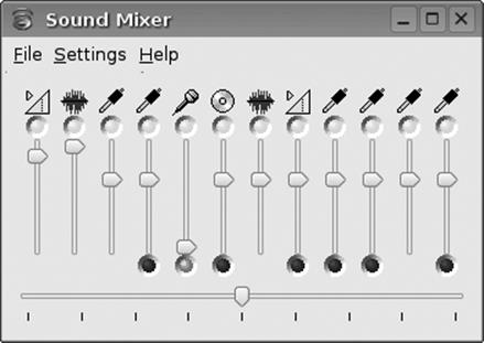
Figure 9-1. KMix

Multimedia Players

Media players are the area with the greatest selection of applications and widest range of features and user interfaces. No one application meets everyone's needs—some aim to be lightweight and fast, whereas others strive to offer the most features. Even within the KDE desktop, for example, a half dozen different players are offered.

If you are running a desktop environment, such as KDE or GNOME, you likely already have at least one media player program. If so, it is recommended that you use this player, at least initially, since it should work correctly with the sound server used by these desktop environments and provide the best integration with the desktop.

When choosing a media player application, here are some of the features you can look for:

§ Support for different sound drivers (e.g., OSS and ALSA) or sound servers (KDE aRts and GNOME esd).

§ An attractive user interface. Many players are "skinnable," meaning that you can download and install alternative user interfaces.

§ Support for playlists, allowing you to define and save sequences of your favorite audio tracks.

§ Various audio effects, such as a graphical equalizer, stereo expansion, reverb, voice removal, and visual effects for representing the audio in graphical form.

§ Support for other file formats, such as audio CD, WAV, and video formats.

Here is a rundown of some of the popular media player applications:

Xmms

Xmms is one popular media player, with a default user interface similar to Winamp. You can download it from http://www.xmms.org if it is not included in your Linux distribution. A screenshot is shown in Figure 9-2.

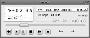
Figure 9-2. Xmms

Xine

Xine is a full-featured audio and video media player that supports many file formats and streaming media protocols. The project is hosted at the following site: http://xine.sourceforge.net. A screenshot is shown in Figure 9-3.

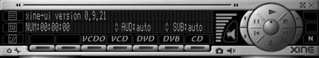
Figure 9-3. Xine

MPlayer

MPlayer is another popular video player that supports a wide range of file formats, including the ability to load codecs from Windows DLLs. It supports output to many devices, using X11, as well as directly to video cards. The project's home page is http://www.mplayer.hu.

Due to legal issues, MPlayer is not shipped by most Linux distributions and so must be downloaded separately.

CD and DVD Burning Tools

If you are running KDE or GNOME, basic CD data and audio burning support is available within the file manager. If you want to go beyond this, or need more help to step you through the process, specialized applications are available.

Note that many of the graphical CD burning applications use command-line tools such as cdrecord and cdrdao to perform the actual CD audio track extraction, ISO image creation, and CD recording. For maximum flexibility, some advanced users prefer to use these tools directly.

X-CD-Roast

One of the first graphical CD burner applications was X-CD-Roast. Although newer applications may offer a more intuitive wizard interface, it is still a reliable and functional program. A screenshot is shown in Figure 9-4.

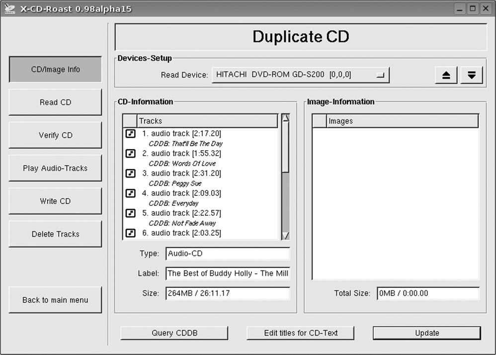
Figure 9-4. X-CD-Roast

K3b

K3b is a popular KDE CD burning tool. It presents a file manager interface similar to popular Windows CD burning utilities such as Easy CD Creator. A screenshot is shown in Figure 9-5. You can find an introduction to K3b in "Burning CDs with K3b," in Chapter 3.

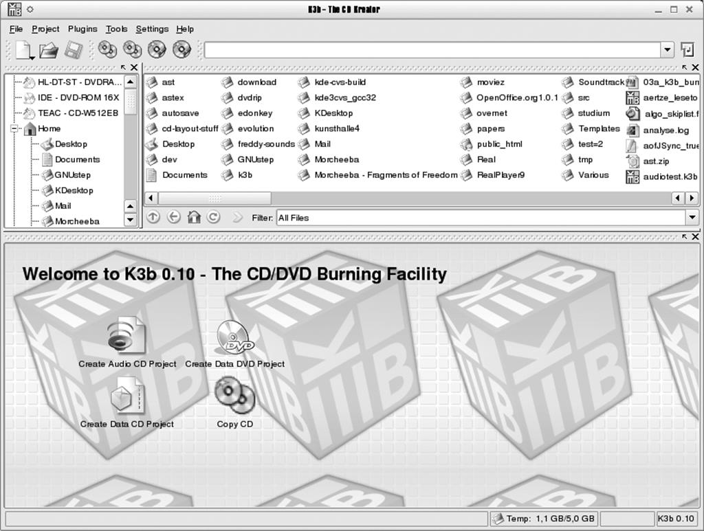
Figure 9-5. K3B

Gcombust

Gcombust is a graphical burner application that uses the Gtk toolkit. The project's home page is http://www.abo.fi/~jmunsin/gcombust. A screenshot is shown in Figure 9-6.

Speech Tools

Speech synthesis and recognition have applications for accessibility and specialized applications, such as telephony, where only an audio path is available.

Speech synthesis devices fall into two major types. Dedicated hardware synthesizers are available that act as a peripheral to a computer and perform the text-to-speech function. These have the advantage of offloading the work of performing the speech conversion from the computer, and tend to offer good-quality output. Software synthesizers run on the PC itself. These are usually lower cost than hardware solutions but add CPU overhead and are sometimes of poor quality if free software is used.

Rsynth

The Rsynth package provides a simple command-line utility called say that converts text to speech. It is included with or available for most Linux distributions.

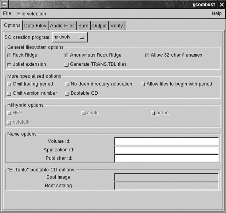
Figure 9-6. Gcombust

Emacspeak

Emacspeak is a text-based audio desktop for visually impaired users. It offers a screen reader that can be used with a hardware or software text-to-speech synthesizer. More information can be found on the project's web site, available here:http://www.cs.cornell.edu/home/raman/emacspeak.

Festival

Festival is a software framework for building speech synthesis systems. It supports multiple spoken languages and can be used to build systems programmed using the shell, C++, Java, and Scheme. The home page for the project is found at http://www.cstr.ed.ac.uk/projects/festival.

IBM ViaVoice

IBM offers a Linux version of the ViaVoice speech SDK that provides both text-to-speech conversion as well as speech recognition. This is a commercial (nonfree) software product.

Image, Sound, and Video Editing and Management Tools

This section describes some of the popular tools for editing images , video, and sound files, as well as managing image collections:

The GIMP

The GIMP is the GNU Image Manipulation Program. It is intended for tasks such as photo retouching, image composition, and image authoring. It has been in active development for several years and is a very stable and powerful program. A screenshot is shown in Figure 9-7. The official web site for the GIMP is http://www.gimp.org.

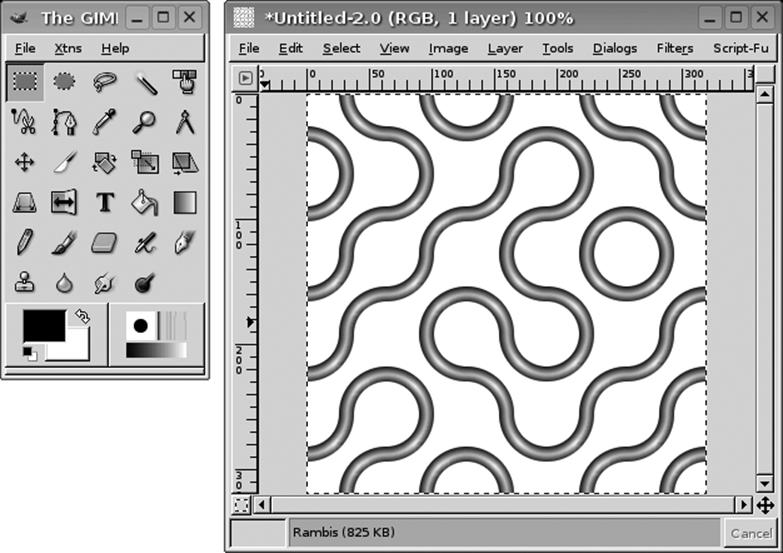
Figure 9-7. GIMP

CinePaint

CinePaint, formerly called Film Gimp, is a painting and image retouching program designed for work with film and other high-resolution images. It is widely used in the motion picture industry for painting of background mattes and frame-by-frame retouching of movies. CinePaint is based on The GIMP but has added features for film editing, such as color depths up to 128 bits, easy navigation between frames, and support for motion picture file formats such as Kodak Cineon, ILM OpenEXR, Maya IFF, and 32-bit TIFF. A screenshot is shown in Figure 9-8. The CinePaint web site is http://www.cinepaint.org.

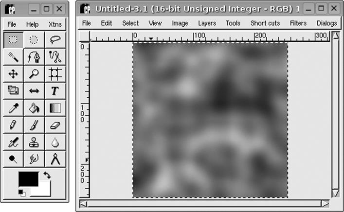
Figure 9-8. CinePaint

Gphoto2

Gphoto2 is a set of digital camera applications for Linux and other Unix-like systems. It includes the libgphoto2 library, which supports nearly 400 models of digital cameras. The other major components are gphoto2, a command-line program for accessing digital cameras, and Gtkam, a graphical application. The project's home page is http://www.gphoto.org. A screenshot of Gtkam is shown in Figure 9-9.

Digikam

Digikam is the KDE digital camera application. It uses libgphoto2 to interface to cameras. A screenshot is shown in Figure 9-10.

Kooka

Kooka is the KDE scanner program. It supports scanners using the SANE library. As well as basic image scanning, Kooka supports optical character recognition of text using several OCR modules. A screenshot is shown in Figure 9-11.

Imaging Tools

A variety of tools are available for acquiring, manipulating, and managing digital images on your computer. In this chapter, we look at some of them.

Image management with KimDaBa

Many applications for viewing images exist, and in our experience, they can be grouped into two main categories: those which are good at generating HTML pages from your image sets, and those which are cool for showing fancy slide shows. The number of applications in both categories is counted in hundreds if not thousands, mostly differing in things that would be considered taste or even religion. You can browse the Linux application sites for your favorite application. Here we focus on an application with a slightly different set of design goals.

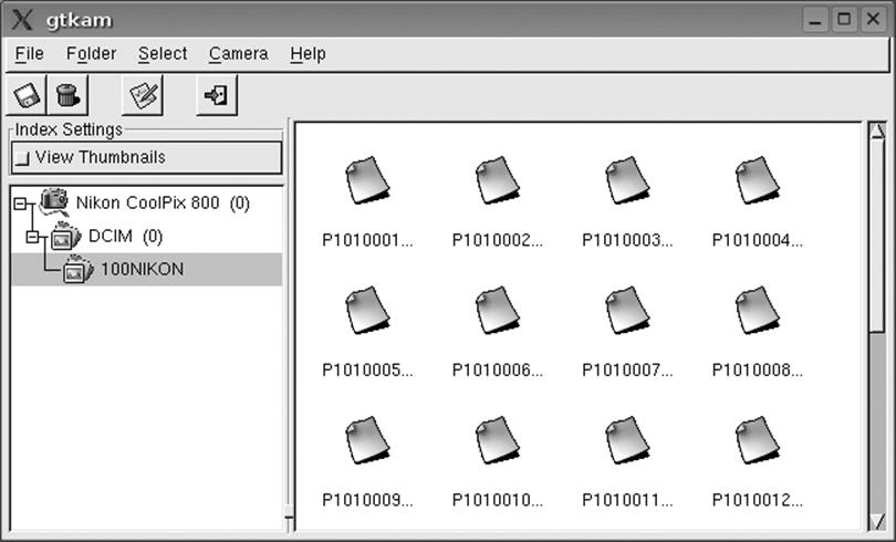
Figure 9-9. Gtkam

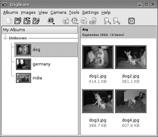
Figure 9-10. Digikam

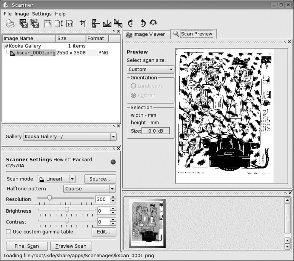
Figure 9-11. Kooka

KimDaBa (KDE Image DataBase) is best explained by the following quote from its home page:

If you are like me you have hundreds or even thousands of images ever since you got your first camera, some taken with a normal camera, others with a digital camera. Through all the years you believed that until eternity you would be able to remember the story behind every single picture, you would be able to remember the names of all the persons on your images, and you would be able to remember the exact date of every single image.

I personally realized that this was not possible anymore, and especially for my digital images—but also for my paper images—I needed a tool to help me describe my images, and to search in the pile of images. This is exactly what KimDaba is all about.

The basic idea behind KimDaBa is that you categorize each image with who is in it, where it was taken, and a keyword (which might be anything you later want to use for a search). When looking at your images, you may use these categories to browse through them. Figure 9-12 shows the browser of KimDaBa.^[*]

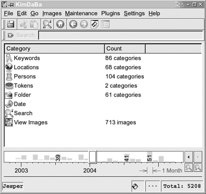
Figure 9-12. Browsing images with KimDaBa

Browsing goes like this: at the top of the list shown in Figure 9-12 you see items for Keywords, Locations, Persons, and so on. To find an image of, say, Jesper, you simply press Persons and, from the list that appears, choose Jesper. Now you are back to the original view with Keywords, Locations, Persons, and so forth. Now, however, you are in the scope of Jesper, meaning that KimDaBa only displays information about images in which Jesper appears. If the number of images is low enough for you to find the image you have in mind, then you may simply choose View Images. Alternatively, repeat the process. If you want to find images with Jesper and Anne Helene in them, then simply choose Persons again, and this time choose Anne Helene. If you instead want images of Jesper in Las Vegas, then choose Locations and, from that view, Las Vegas.

There is no such thing as a free lunch. For KimDaBa this means that you need to categorize all your images, which might be a rather big task — if you have thousands of images. KimDaBa is, however, up to this task — after all, one of its main design criteria is to scale up to tens or even hundreds of thousands of images.

There are two ways of categorizing images in KimDaBa, depending on your current focus, but first and foremost let's point out that the categorizing tasks can be done step by step as you have time for them.

The first way of categorizing images is by selecting one or more images in the thumbnail view (which you get to when you press View Images), and then press the right mouse button to get to the context menu. From the context menu, either choose Configure Images One at a Time (bound to Ctrl-1) or Configure All Images Simultaneously (bound to Ctrl-2).

Configure All Images Simultaneously allows you to set the location of all images from, say, Las Vegas with just a few mouse clicks, whereas Configure Images One at a Time allows you to go through all the images one by one, specifying, say, who is in them.

Figure 9-13 shows the dialog used for setting properties for the images. In this dialog you may either select items from the list boxes or start typing the name in question—KimDaBa will offer you alternatives as you type. (In the screenshot, I only typed J, and KimDaBa thus found the first occurrence that matched.)

The alternative way of specifying properties is to do it while you view your images (e.g., as a full-screen slide show). In this mode, you simply set a letter token on the image by pressing the letter in question. This usage is intended for fixing annotations later on—say you are looking at your images and realize that you forgot to mark that Jesper is in a given image. Once you have set a number of tokens, you can use these for browsing, just as you use persons, locations, and keywords. What you typically would do is simply to browse to the images with a given token, and then use the first method specified previously to set the person missing in the images.

Once you have annotated all your images, you can drive down memory lane in multiple ways. As an appetizer, here is a not-so-uncommon scenario derived from personal use of KimDaBa: you sit with your girlfriend on the living-room sofa, discussing how much fun you had in Mallorca during your vacation in 2000, and agree to grab your laptop to look at the images. You choose Holiday Mallorca 2000 from the keyword category, and start a slide show with all the images. As you go on, you see an image from when you arrived home. On that image is an old friend who you haven't talked to in a long time. In the full-screen viewer, you press the link with his name (all the information you typed in is available during viewing in an info box). Pressing his name makes KimDaBa show the browser, with him in scope. Using the date bar, you now limit the view to only show images of him from 1990 to 2000. This leads you to some images from a party that you attended many years ago, and again the focus changes, and you are looking at images from that party. Often, you end up getting to bed late those evenings when you fetch the laptop.

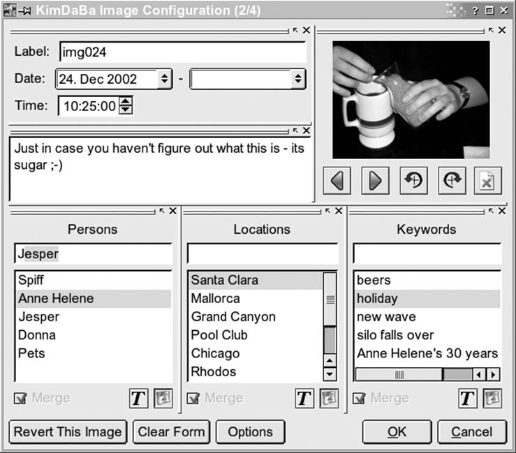
Figure 9-13. Configuring KimDaBa

Image manipulation with the GIMP

Introduction. The GIMP is the GNU Image Manipulation Program. It is intended for tasks such as photo retouching, image composition, and image authoring. It has been in active development for several years and is a very stable and powerful program.

The GIMP's home is http://www.gimp.org, the online manual is available from http://docs.gimp.org, and additional plug-ins to expand GIMP's features can be found at http://registry.gimp.org.

It is possible to use GIMP as a simple pixel-based drawing program, but its strength is really image manipulation. In this book we present a small selection of useful tools and techniques. A complete coverage of the GIMP would require a whole book, so read this only as a teaser and for inspiration to explore GIMP.

At the time of writing the current version of GIMP was 2.2. Minor details in the feature set and user interface will be different in other versions, but the overall idea of the application is the same.

Selection tools. When GIMP is started, it shows the toolbox window, as seen in Figure 9-14. The upper part of the toolbox contains a number of buttons, each of which represents a tool. There is also a menubar with menus for creating new images, loading, saving, editing preferences, and so on. Below the buttons is a section showing the current foreground and background colors, selected pen, and so on. The lower part of the window shows the options for the current tool.

To create a new image, choose File → New. This gives us a blank image to use for experimenting with the tools.

The first five tools are selection tools: rectangle, ellipse, freehand, magic wand, by color, and shape-based selection. A selection is an area of the image that almost any tool and filter in GIMP will work on—so it is an important concept. The current selection is shown with "marching ants." You can show and hide the marching ants with Ctrl-Z.

The first three selection tools are, except for the shape of the selection made, quite similar. While dragging out a rectangular or elliptical selection, it is possible to keep a constant aspect ratio by holding down the Shift key. In the option window for each selection tool, it is possible to choose a selection mode to add to an existing selection, subtract from one, replace the current selection, and intersect with one.

All selection tools have a feather parameter that will control how soft the edges of the selection are. See Figure 9-15 for an example.

The magic wand allows you to click on a pixel in the image and thereby select a contiguous area around the pixel with similar color. Use the threshold slider to control how similar the colors must be. Selection by color works like the magic wand, but it selects all pixels with similar value — contiguous or not. Finally, selection by shapes allows you to place points in the image and try to connect the points with curves that follow edges in the image. When you have selected enough points to contain an area, click in the middle of that area to convert the traced curve to a selection.

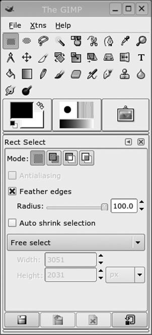
Figure 9-14. GIMP toolbox

Painting and erasing tools. To paint in an image, the Pencil, Paintbrush, Airbrush and Ink tools can be used. They differ in the way the shapes you draw look: Pencil paints with hard edges, and Paintbrush with soft edges, Airbrush paints semitransparently and Ink thickens the line when you paint slowly and thins the line when you paint quickly.

To fill in an area, make a selection and use the paintbucket or gradient fill tool to fill it with color. Selecting the pen style, color, and/or gradient can be done by clicking the controls in the middle of the toolbox window.

Some people have trouble drawing a straight line in GIMP, but since you have this clever book in your hands, you will know the secret: select one of the drawing tools, place the cursor where you want the line to start, press and hold Shift, and then move the mouse to where the line should end and click once with the left mouse button. Now either do the same again to draw another line segment or release the Shift key and enjoy your straight line.

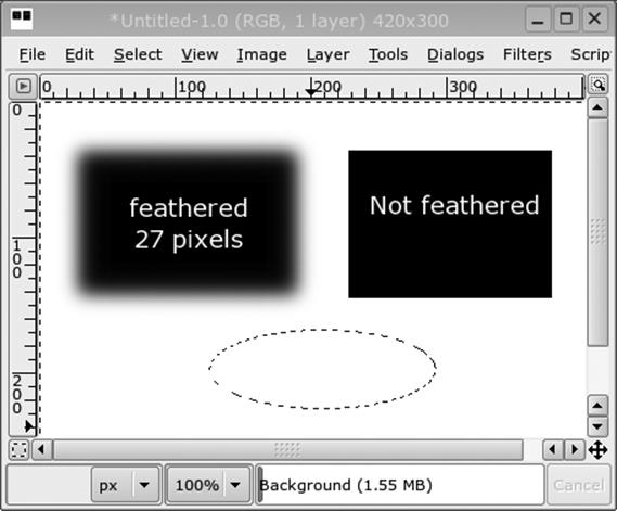
Figure 9-15. GIMP selections

If you make a mistake, use the most often used keyboard shortcut in GIMP: Ctrl-Z to undo. Multiple levels of undo are available. There is also an eraser tool that allows you to selectively erase pixels.

Everything you do with the painting tools will be confined to the currently selected area if there is a selection.

Photo retouching tools . The tools in this section are mostly for modifying digital photos in subtle (and not so subtle) ways. The Clone tool is very useful to remove blemishes from a photo. It works by first Ctrl-clicking in an image to set the source point, and then painting somewhere in an image. You will now paint with "copies" of the source area. Figure 9-16 shows the upper-right corner of a landscape photo that got a bit of the roof from a house into the frame. The left image is the original, and the right one has the undesired feature removed by using the clone tool with some other part of the clouds as the source area.

The last tool in the toolbox is the Dodge and Burn tool. It is used to lighten (dodge) and darken (burn) parts of an image by drawing on it. This tool can be used to finetune areas with shadows or highlights.

Color adjustment. During postprocessing of digital photos, it can be very useful to adjust the overall appearance of the light, color, and contrast of a photo. GIMP supports quite a number of tools for this. They are available in the Layer/Colors context menu.

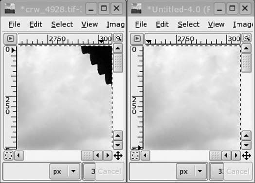
Figure 9-16. GIMP clone tool

One of the more useful tools is the Levels tool. It allows you to adjust the black and white points of an image. Figure 9-17 shows a photo shot in harsh lighting conditions. It has low contrast and looks hazy.

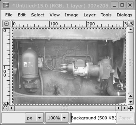
Figure 9-17. Original photo

Let's fix that problem using the Levels dialog! Open the dialog for the Levels tool by choosing Levels from the menu. The dialog can be seen in Figure 9-18.

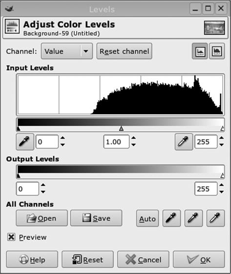
Figure 9-18. Levels dialog

The diagram seen under "Input Levels" is a histogram of the brightness values in the image. The left end of the histogram represents black, and the right end white. We see that that the lower 40% of the histogram is empty—this means that we are wasting useful dynamic range. Below the histogram are three triangular sliders. The black and the white ones are for setting the darkest and brightest point in the image, and the gray one is for adjusting how values are distributed within the two other ones. We can move the black point up as shown in Figure 9-19 to remove the haziness of the image. The result is shown in Figure 9-20.

Contrast enhancement can be done either with the Brightness-Contrast tool or with the Curves tool. The former is quite basic consisting of two sliders, one for brightness and one for contrast; the latter allows much more control. Figure 9-21 shows an original image and two modified versions with different curves applied. The middle image has the contrast-enhancing curve shown in Figure 9-22 applied, and the right image has the contrast-decreasing curve shown in Figure 9-23 applied. The curves describe a mapping from pixel values onto itself. A straight line at a 45-degree slope is the identity mapping; anything else will modify the image. Best results are obtained if you only deviate a little bit from the 45-degree straight line.

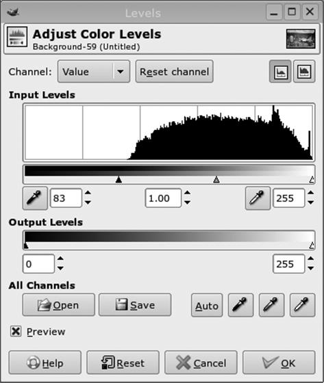
Figure 9-19. Levels dialog

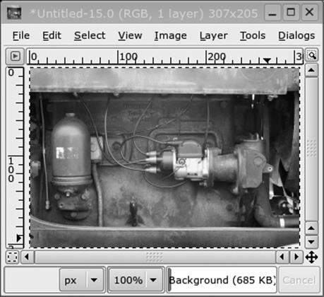
Figure 9-20. Level adjusted

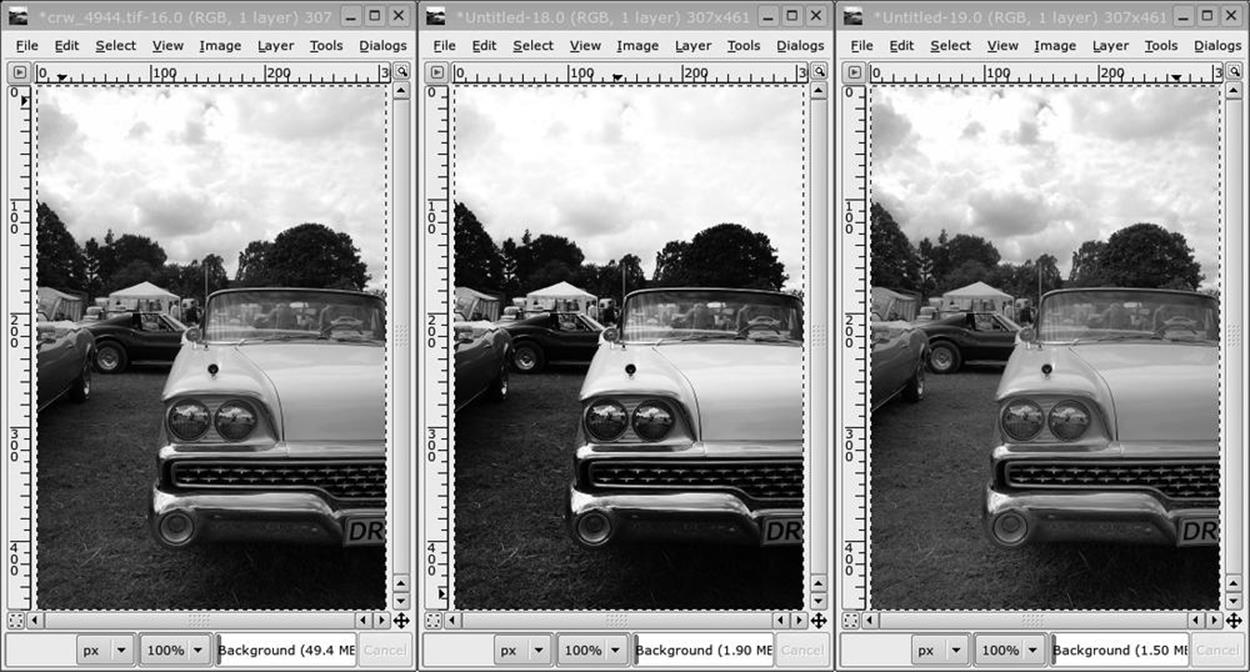
Figure 9-21. Curve adjusted

Colors can be changed with several tools, such as the Color Balance and Hue-Saturation tools. The Levels and Curves tools can also be set to operate on individual color channels to achieve various effects. But there is also another tool available: the Channel Mixer. Unlike the other tools this is located in the Filters/Colors/Channel Mixer context menu. The Channel Mixer can be used to create a weighted mix of each color channel (red, green, and blue) for each of the output channels. It is particularly useful for converting color images to monochrome, often giving better results than simply desaturating the image. Figure 9-24 shows the Channel Mixer, and Figure 9-25 shows two monochrome versions of the same color image. The upper one is simply desaturated, and the lower one is based only on the blue channel and seems to emphasize the bird rather than the background. When judging how to convert a color image to monochrome, it can be helpful to examine each color component individually. See the paragraph about channels for more about this.

Layers and channels. The most convenient way to access layers and channels is through the combined layers, channels, paths, and undo history window. It can be accessed by right-clicking in the image's windows and selecting the Dialogs → Create New Dock → Layers, Channels & Paths menu item. Layers and channels allow you to view and manipulate different aspects of your images in a structured way.

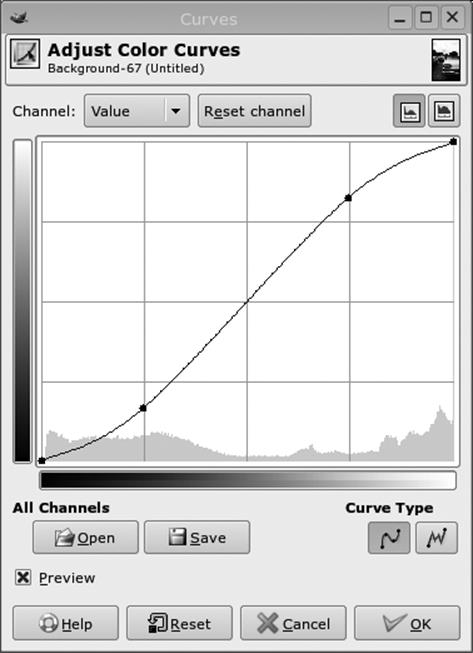
Figure 9-22. Contrast-enhancing curve

Channels

An image is made up from one or more channel(s). True color images have three color channels, one for each of the red, green, and blue components. Index-colored and grayscale images have only one color channel. All types can have an optional alpha channel that describes the opacity of the image (white is completely opaque; black is completely transparent). By toggling the eye button for each channel, you can selectively view only a subset of the channels in an image. Channels can be selected or deselected for manipulation. For normal operation, all color channels are selected, but if you only want to paint into the red channel, for example, deselect the other channels. All drawing operations will then only affect the red channel. This can, for example, be used to remove the red flash reflection in your subjects' eyes. You can add additional channels to an image using the buttons at the bottom of the dialog. A very useful feature is that you can save a selection as a channel and convert a channel to a selection. This allows you to "remember" multiple selections for later use, and it makes it easier to fine-tune a selection because you can paint into a channel to add or remove areas to a selection. Figure 9-26 shows the Channel tab in the combined Layers, Channels dialog. The green and blue channels are visible, and the green channel is selected for editing.

Layers

Layers are a very powerful feature of the GIMP. Think of layers as a way of stacking multiple images on top of each other, affecting each other in various ways. If a layer has an alpha channel, the layers beneath it will show through in transparent areas of the layer. You can control the overall opacity of a layer by using the opacity slider shown in the dialog. Use the buttons at the bottom of the dialog to create, duplicate, and delete layers and to move layers up and down the stacking order. You can assign a name to a layer by right-clicking it and choosing Edit Layer Attributes. Figure 9-27 shows the Layers tab in the Layers, Channels dialog with an image loaded and two duplicate layers created.

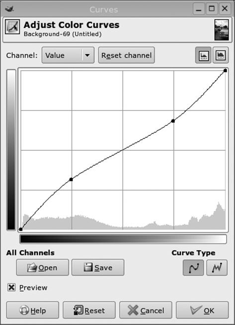
Figure 9-23. Contrast-decreasing curve

Recall the image of the car from the curves example. The ground and car looked most interesting with the high-contrast curve, but the sky lost detail with this curve—it looked better with the low-contrast curve because it pulled out detail from the bright sky. Let us try to combine those two approaches. We'll leave the lowest layer alone — it will serve as a reference. Rename the middle layer "Ground" and the topmost one "Sky." Now make only the Ground layer visible, select it, and use the Curves tool to enhance contrast. Then make the topmost layer visible, select it, and apply a low-contrast curve to it. Now we need to blend the two layers together. To do this, we add a layer mask to the topmost layer, but before we do that, we want to get a good starting point for the mask. Use the magic wand selection tool to select as much of the sky as possible without selecting any of the trees, cars, or the ground. Remember that Shift-clicking adds to a selection. When most of the sky is selected, right-click on the topmost layer and choose Add Layer Mask and then choose Selection in the dialog that pops up. Don't worry if the selection doesn't align perfectly at the pixel level with the horizon — we can fix that later. Press Ctrl-Shift-A to discard the current selection—we don't need it any more. Now the Layers dialog should look like Figure 9-28.

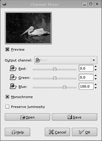
Figure 9-24. Channel Mixer

By clicking on either the layer thumbnail or the layer mask thumbnail, you can choose which one of them you want to edit. Choose the layer mask and zoom in on the boundary between the trees and the sky. Now the mask can be adjusted by simply painting on the image with a black or white pen. White makes the sky show through and black makes the trees show through. To see the mask itself instead of the image, right-click the mask in the Layers dialog and choose Show Mask. The result should look something like Figure 9-29.

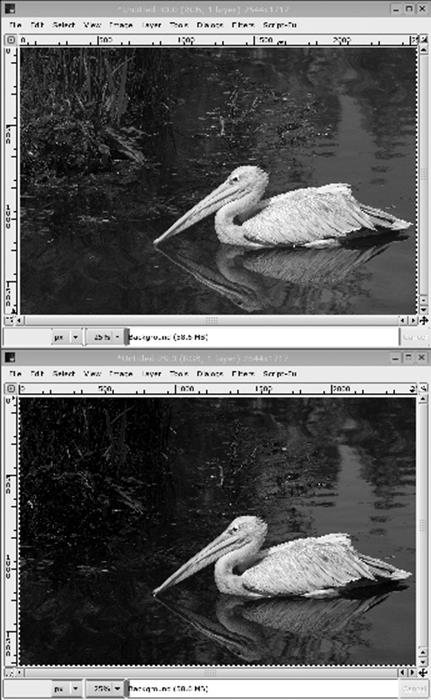
Figure 9-25. Channel Mixer example

So far we've only been using layers in Normal mode, but there are other modes as well. The other modes make a layer interact with the layers below it in interesting ways. It is possible to make the pixel values in a layer burn, dodge, multiply, and so forth, with the pixel values of the layer below it. This can be very powerful when used properly. Figure 9-30 shows the image from before with a new transparent layer added on top of it. This new layer contains the result of selecting a rectangle slightly smaller than the whole image, feathering the selection with a large radius (10% of the image height), inverting it, and filling out the selection with black paint. The mode of the layer is set to Overlay, which causes a slight darkening of the layers below it around the black areas near the borders. The effect looks as if the photo were taken with an old or cheap camera and adds to the mood of the scene. If we had used the Normal mode instead of Overlay, the effect would have been too much and looked unnatural. Try experimenting with the different modes yourself!

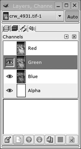
Figure 9-26. Channels dialog

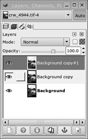
Figure 9-27. Layers dialog

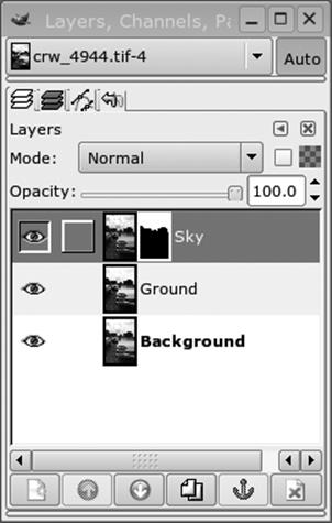
Figure 9-28. Layers and mask

Filters. The final major aspect of GIMP we cover here is its filters. Filters are effects that can be applied to an entire image or a selection. GIMP is shipped with a large number of different filters, and it is possible to plug in new filters to extend the capabilities of GIMP. Filters are located in the right mouse button Filters menu. The Channel Mixer is an example of such a filter. We discuss two useful filters, Gaussian Blur and Unsharp Mask, and apply them to the image from the previous example.

Gaussian Blur

This filter provides a nice smooth blurring effect. Try it with different blur radius settings. The IIR-type Gaussian blur seems to look better than RLE with most images.

For our example we are not going to blur the actual image. Instead, we are going to smooth out the transition between the high- and low-contrast layers. Do this by selecting the layer mask in the sky layer and applying Gaussian Blur. A radius of 8 seems to work well here. Zoom in on the border between the trees and the sky, and don't be afraid to experiment — you can always press Ctrl-Z to undo and try again. Figure 9-31 shows a closeup of before and after applying Gaussian Blur to the mask. The effect is subtle, but important for making the two layers blend seamlessly.

Unsharp Mask

Despite its name, Unsharp Mask is a filter for enhancing the perceived sharpness of images. It offers more control and often provides more pleasing results than the simple Sharpen filter. Unsharp Mask works like this: first it makes an internal copy of your image and applies a Gaussian blur to it. Then it calculates the difference between the original and the blurred image for each pixel, multiplies that difference by a factor, and finally adds it to the original image. The idea is that blurring affects sharp edges much more than even surfaces, so the difference is large close to the sharp edges in the image. Adding the difference back further emphasizes those sharp edges. The Radius setting for Unsharp Mask is the radius for the Gaussian blur step, the Amount is the factor that the differences are multipled by, and the Threshold setting is for ignoring differences smaller than the chosen value. Setting a higher threshold can help when working with images with digital noise in them so we don't sharpen the noise.

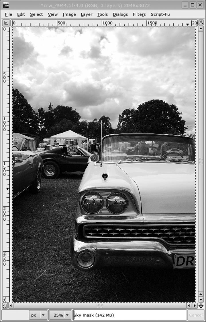
Figure 9-29. Two layers

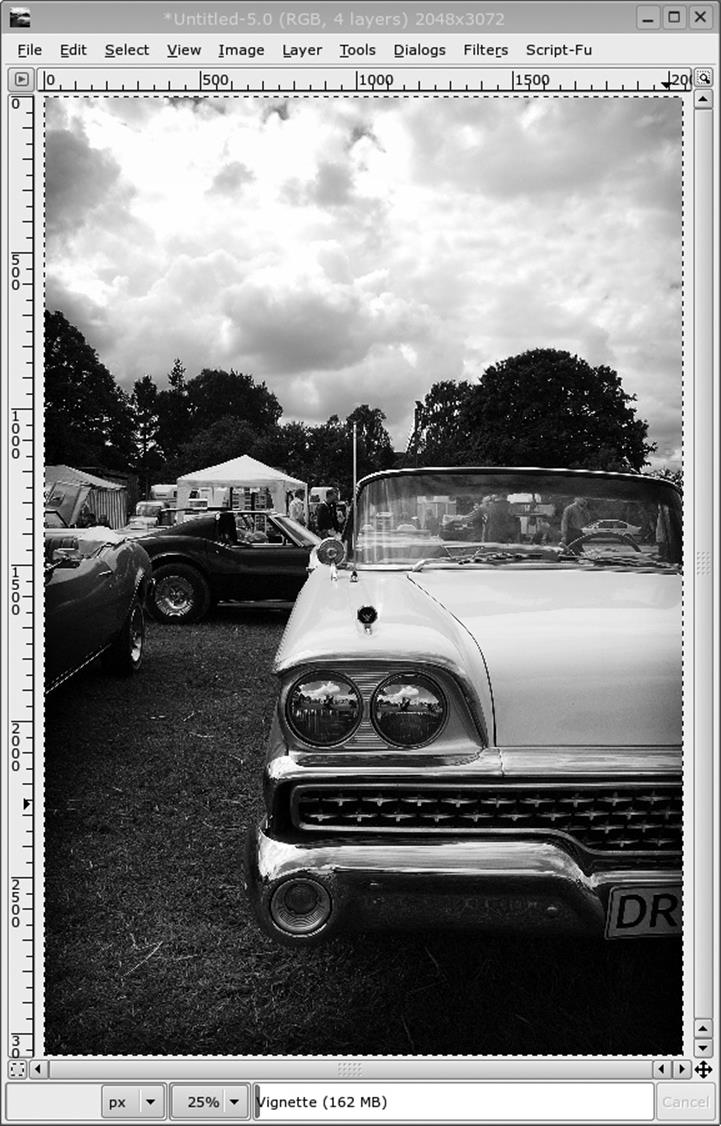
Figure 9-30. Two layers

Looking at our example with the sky and car again, we notice that the high-contrast part lost some details in the shadows when we pulled up the contrast. This can also be remedied with Unsharp Mask. To do this, we apply Unsharp Mask with a high radius and low amount. This technique is called "local contrast enhancement." Start out by making a copy of the whole image by pressing Ctrl-D and merging all layers in the copy. This is done by choosing Image → Flatten Image from the context menu. Then we want to scale the image for screen viewing. Open the scaling dialog by choosing Image → Scale Image from the context menu and choosing a suitable size and the bicubic (best) scaling algorithm. Now we are ready to apply Unsharp Mask for local contrast enhancement. A radius of 25, an amount of 0.15, and threshold of 0 seems to look good.

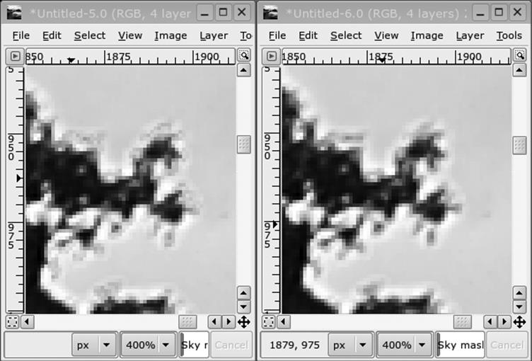
Figure 9-31. Blurring the mask — before and after

Finally, we want to sharpen up the edges a bit. To do this, we apply Unsharp Mask with a small radius (0.5) and higher amount (0.5) and with a threshold of 6. Figure 9-32 shows the unsharpened image on the left, the image with local contrast enhancement applied in the middle, and the image with the final sharpening pass applied on the right.

Recording Tools

If you want to create your own MP3 files, you will need an encoder program. There are also programs that allow you to extract tracks for audio CDs.

Although you can perform MP3 encoding with open source tools, certain patent claims have made the legality of doing so questionable. Ogg Vorbis is an alternative file format and encoder that claims to be free of patent issues. To use it, your player program needs to support Ogg Vorbis files because they are not directly compatible with MP3. However, many MP3 players, such as Xmms, support Ogg Vorbis already; in other cases, there are direct equivalents (such as ogg123 for mpg123). For video, Ogg has developed the Ogg Theoris codec, which is free and not encumbered by any patents.

This section lists some popular graphical tools for recording and manipulating multimedia.

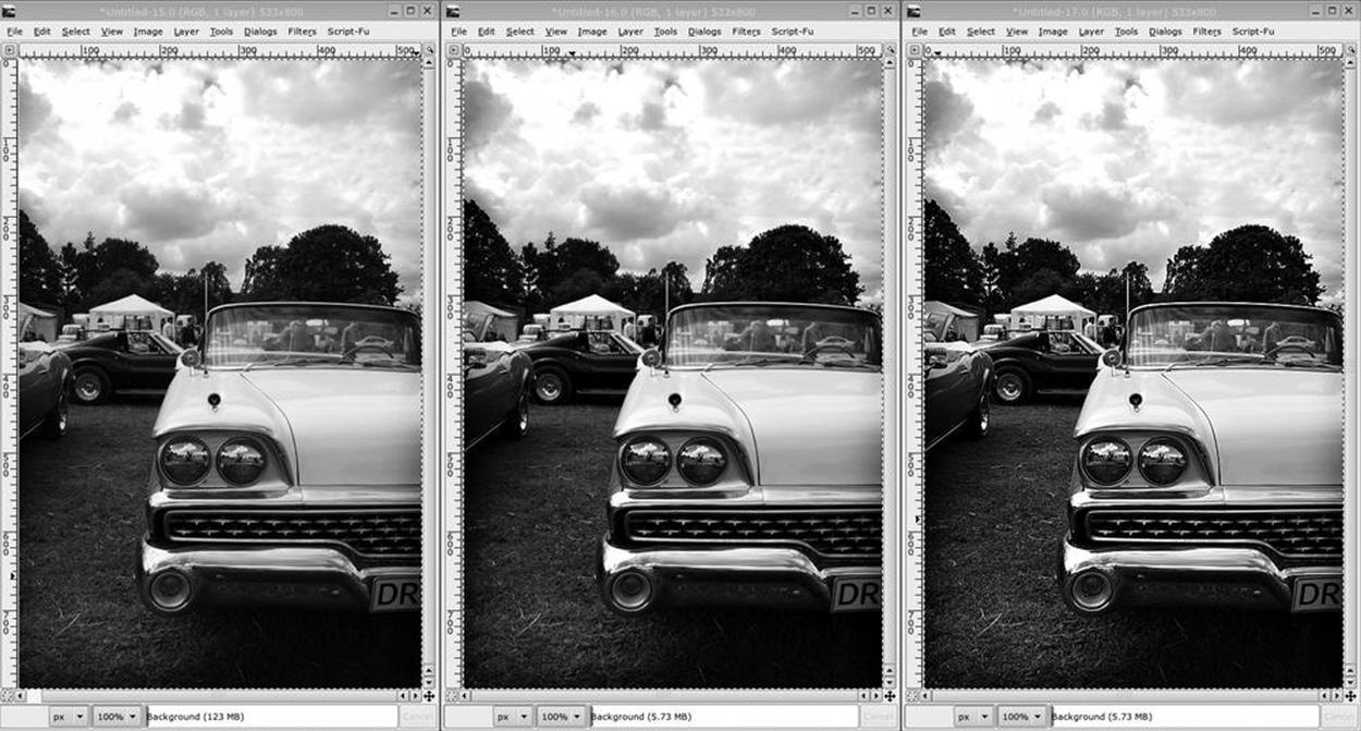
Figure 9-32. Two passes of Unsharp Mask

Krec

KDE includes Krec as the standard sound recorder applications. You can record from any mixer source, such as a microphone or CD, and save to a sound file. Although it offers some audio effects, it is intended as a simple sound recorder application. A screenshot is shown in Figure 9-33.

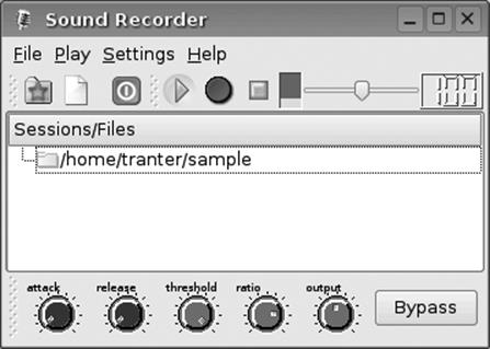
Figure 9-33. Krec

Audacity

Audacity is an audio editor that can record and play back sounds and read and write common sound file formats. You can edit sounds using cut, copy, and paste; mix tracks; and apply effects. It can graphically display waveforms in different formats.

A screenshot is shown in Figure 9-34. The project home page is http://audacity.sourceforge.net.

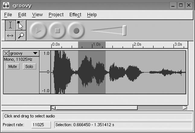
Figure 9-34. Audacity

Ardour

Ardour is a full-featured digital audio workstation designed to replace analog or digital tape systems. It provides multitrack and multichannel audio recording capability, mixing, editing, and effects. A screenshot is shown in Figure 9-35. The project home page is http://ardour.org.

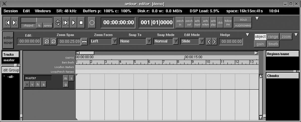
Figure 9-35. Ardour

Freevo

Freevo is an open source home theater platform based on Linux and open source audio and video tools. It can play audio and video files in most popular formats. Freevo can be used as a standalone personal video recorder controlled using a television and remote, or as a regular desktop computer using the monitor and keyboard.

A screenshot is shown in Figure 9-36. The project home page is http://freevo.sourceforge.net.

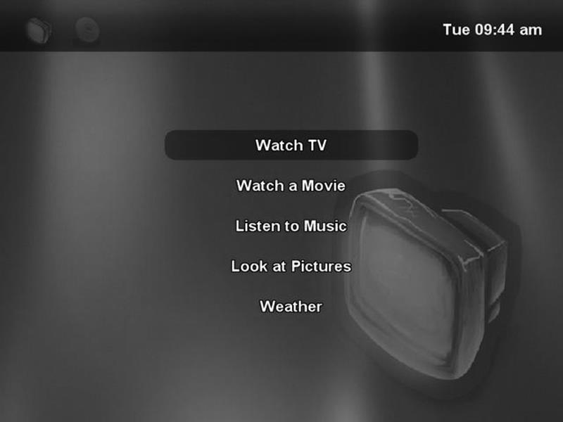
Figure 9-36. Freevo

MythTV

MythTV is a personal video recorder (PVR ) application that supports a number of features, including

§ Watching and recording television

§ Viewing images

§ Viewing and ripping videos from DVDs

§ Playing music files

§ Displaying weather and news and browsing the Internet

§ Internet telephony and video conferencing

A screenshot is shown in Figure 9-37. The MythTV home page is http://mythtv.org.

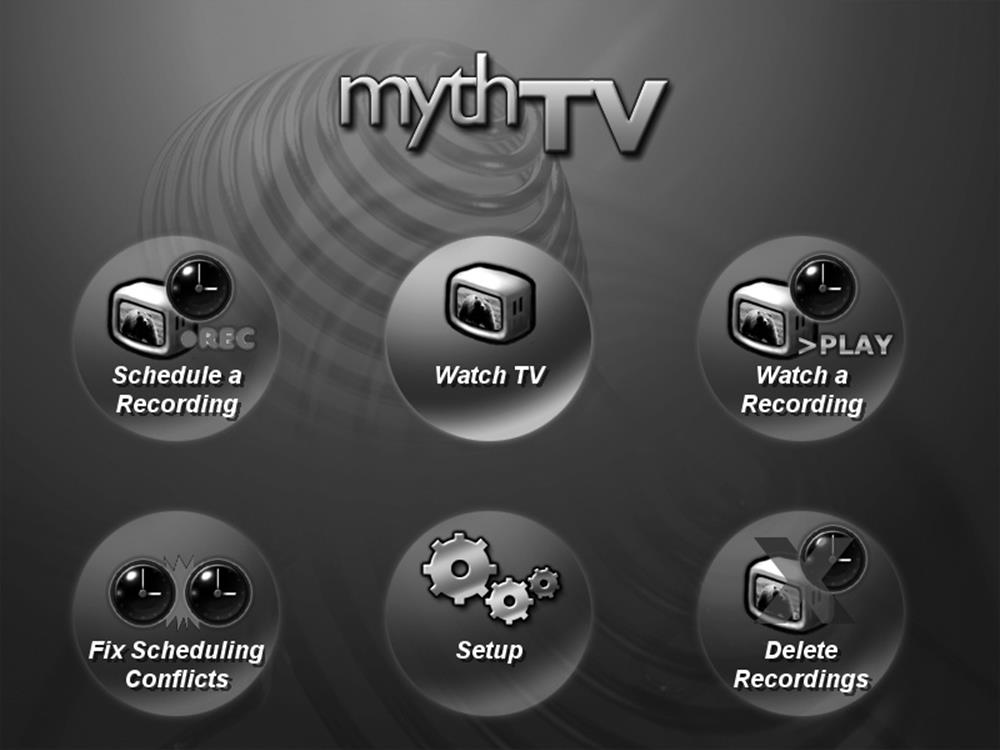
Figure 9-37. MythTV

Music Composition Tools

Many applications are available that help music composers.

MIDI sequencers allow a composer to edit and play music in MIDI format. Because MIDI is based on note events, tracks, and instruments, it is often a more natural way to work when composing music than directly editing digital sound files.

Scoring programs allow composers to work with traditional music notation and produce typeset sheet music. Some support other notation formats such as tablature for guitar and other instruments.

Some programs combine both MIDI sequencing and scoring, or can work with various standardized file formats for musical notation.

Brahms

Brahms is a KDE-based MIDI sequencer application that allows a composer to edit tracks and play them back. You can work with MIDI events or a traditional music score using different editor windows. A screenshot is shown in Figure 9-38. The project home page ishttp://brahms.sourceforge.net.

Rosegarden

Rosegarden is an audio and MIDI sequencer, score editor, and general-purpose music composition and editing environment. It allows you to work with MIDI events or music notation. It is integrated with other KDE applications and has been localized into about 10 languages.

A screenshot is shown in Figure 9-39. The project home page is http://www.rosegardenmusic.com.

LilyPond

LilyPond is a music typesetter that produces traditional sheet music using a high-level description file as input. It supports many forms of music notation constructs, including chord names, drum notation, figured bass, grace notes, guitar tablature, modern notation (cluster notation and rhythmic grouping), tremolos, (nested) tuplets in arbitrary ratios, and more.

LilyPond's text-based music input language support can integrate into LAT_EX, HTML, and Texinfo, allowing documents containing sheet music and traditional text to be written from a single source. It produces PostScript and PDF output (via T_EX), as well as MIDI.

The project home page is http://lilypond.org. There is a graphical front end to LilyPond called Denemo.

Internet Telephony and Conferencing Tools

Telephony over the Internet has recently become popular and mainstream. Using VOIP (Voice Over IP) technology, audio is streamed over a LAN or Internet connection. SIP (Session Initiation Protocol) is a standard for setting up multimedia sessions (not just audio). Either a sound card and microphone or dedicated hardware resembling a traditional telephone can be used. Internet telephony has a number of advantages, but the main one is cost—many users today have a full-time high-speed Internet connection that can be used to connect to anyone else in the world with compatible software. With a suitable gateway, you can make a call between a VOIP phone and the public telephone network.

There are many VOIP applications for Linux. KPhone is one popular KDE-based one. As well as audio, it supports instant messaging and has some support for video. The project's home page is http://www.wirlab.net/kphone.

There are also commercial applications that use proprietary protocols or extensions to protocols. One example is Skype, which offers a free client but requires subscription to a service to make calls to regular phones through a gateway. Skype can be found at http://www.skype.com.

H.323 is a standard for video conferencing over LANs. It is supported by Microsoft NetMeeting, which is included with Microsoft Windows. H.323-compliant applications are available on Linux, the most notable being GnomeMeeting. The project's home page ishttp://www.gnomemeeting.org.

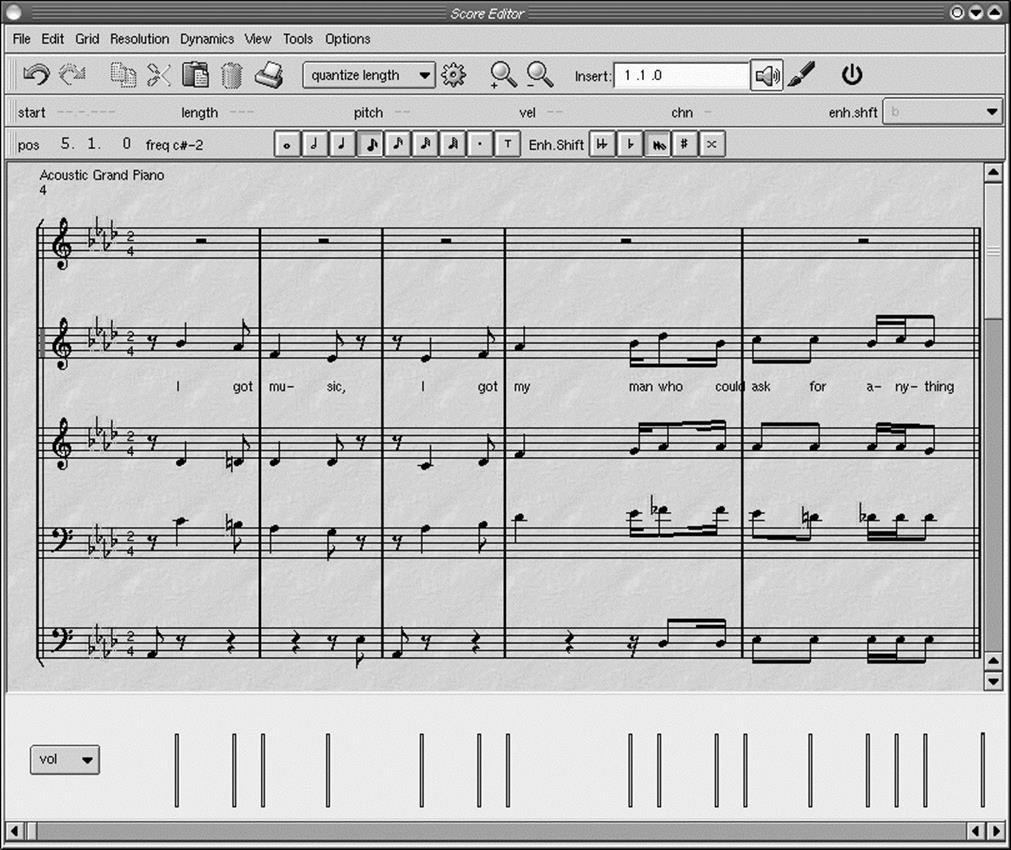
Figure 9-38. Brahms

Browser Plug-ins

Browser plug-ins allow data types other than HTML to be presented in your web browser. Some of these qualify as multimedia. They can be divided into three categories:

§ Plug-ins that come with the browser or are available from the same source as the browser (e.g., Mozilla or Firefox).

§ Native plug-ins from third parties, such as Adobe Acrobat, usually available at no cost although they may be closed source.

§ Windows plug-ins that can run inside some Linux browsers using CodeWeaver's CrossOver (Wine) technology. This category includes plug-ins such as Apple QuickTime, Windows Media Player, and Adobe Shockwave. Many of these are not available as native Linux plug-ins.

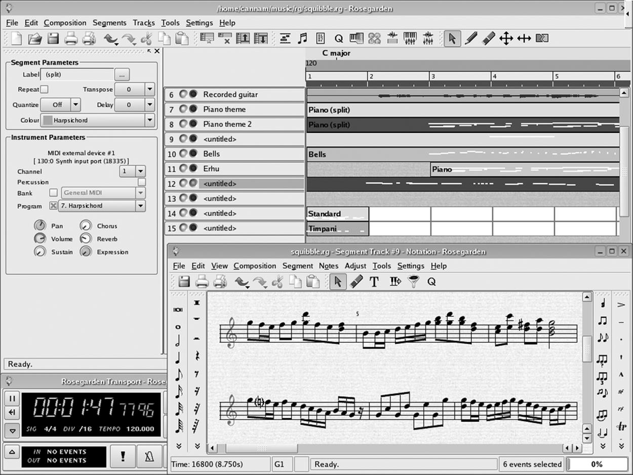
Figure 9-39. Rosegarden

The Netscape plug-in format is supported by Netscape, Mozilla, and some other browsers derived from Mozilla, such as FireFox. Netscape plug-ins are also supported by the KDE project's Konqueror browser.

Putting It All Together

This chapter has talked about a lot of different multimedia tools. Although most of these tools are straightforward to use and perform a well-defined function on their own, more powerful tasks can be performed by combining tools. Let's look at a real-life example.

I like to collect and restore old vacuum tube radios from the 1930s through 1950s. After I have restored a radio to working condition I like to display it. But when I turn it on, hearing the local sports or talk radio station doesn't seem appropriate. Wouldn't it be fun to hear some old radio shows from the era in which the radio was made coming out of the radio?

Lots of old-time radio broadcasts are available as free downloads on the Internet. I can download a number of these to my computer. It is also possible to buy CDs of old radio programs. I might even have an old vinyl record or cassette tape of old radio shows. Using Audacity and connecting a turntable or tape player to my sound card's audio input, I can convert them to sound files. The files can have some simple editing and processing done to clean them up, and they can be converted to MP3 format.

If I want to listen to them on my computer, I can use Juk to arrange them in playlists of my favorite programs arranged by type and have hours of continuous music or radio shows. I can save the MP3 files to my portable MP3 player to listen to when I am away from the computer, or burn them to a CD to listen to with a portable CD player.

Using a low-power AM transmitter, I can legally broadcast programming throughout my home. An inexpensive AM transmitter is available from a number of sources and connects either to the sound card output of my computer or a CD player, and can broadcast vintage radio programs on the AM band to radios within the house. Now when I turn on that old radio, I can hear Burns and Allen, The Shadow, or some swing music from the 1940s. I might even be able to convince the more gullible visitors to my radio room that old radios can still pick up old radio programs.