MICROSOFT BIG DATA SOLUTIONS (2014)

Part V. Big Data and SQL Server Together

In This Part

· Chapter 10: Data Warehouses and Hadoop Integration

· Chapter 11: Visualizing Big Data with Microsoft BI

· Chapter 12: Big Data Analytics

· Chapter 13: Big Data and the Cloud

· Chapter 14: Big Data in the Real World

Chapter 10. Data Warehouses and Hadoop Integration

What You Will Learn in This Chapter:

· Understanding the Current “State of the Union”

· Learning About the Challenges Faced with the Traditional Data Warehouse

· Discovering Hadoop's Impact on Data Warehouses and Design

· Introducing Parallel Data Warehouse

· Finding Out About PDW's Architecture

· Grasping the Concepts Behind Project Polybase

· Gaining Insight on How to Use Polybase in Solutions

· Looking into the Future for Polybase

There has never been a more exciting time to be working in the analytics and data warehousing space; and it most certainly is a space. Data warehouses should be considered to be a place for free thinking—logical entities that holistically span the business, not physical beings constrained by limits of today's technology and yesterday's decisions. The aspiration for the new world of data is liberty: seamless, friction free-integration across the enterprise and beyond.

Therefore, we start by taking a deeper look at the emerging relationship between data warehouses and Hadoop. The current methods using Sqoop offer limited value, but both data warehouse vendors and Hadoop need more. More importantly, business has demanded more. More so than ever, data warehouse vendors have really had to up their game to demonstrate their value and thought leadership to the enterprise in the face of the disruptive technology that is Hadoop.

This chapter focuses on the changes Microsoft has been making to their data warehouse offerings to address the challenges faced by data warehouses and also how they are embracing Hadoop, offering industry-level innovation to Hadoop integration with Project Polybase. Let's get started.

State of the Union

When I think about data warehouses, I am often reminded of this famous Donald Rumsfeld quote:

“There are known knowns; there are things we know that we know. There are known unknowns; that is to say, there are things that we now know we don't know. But there are also unknown unknowns—there are things we do not know we don't know.”

In my mind, I compartmentalize this quote into Table 10.1.

Table 10.1 Compartmentalizing Data Warehousing

Traditional data warehouses have been focused on historical analysis and performance. In other words, we are looking back. At best, we get as far as the known unknowns. The fact that we can model, shape, and organize the data is evidence of the fact that we know what we are looking for. Although this is helpful to operationally optimize a business process, it actually isn't “intelligence” and it isn't transformative. It's not going to help us get close to answering the unknown unknowns. In actuality, the very fact that we've modeled the data may make it impossible, because in so doing we may have lost subtle nuances in the data that only exist in its raw, most granular form.

However, the beauty of the new world of data warehousing and analytics is that it is all about answering questions. In recent times, advances in technology have enabled us to ask bigger, more exciting, interesting, and open-ended questions—in short big questions. The question is what puts the big in big data. What's more, we can now answer those big questions.

Challenges Faced by Traditional Data Warehouse Architectures

What is a traditional architecture when it is at home? Every warehouse I come across certainly has some distinguishing features that make it different or special. However, many of these warehouses usually share one very common element in their architecture: they are designed to a symmetric multiprocessor (SMP) architecture; that is, they are designed to scale up. When you exceed the capabilities of the existing server, you go out and buy a bigger box. This is a very effective pattern for smaller systems, but it does have its drawbacks. These drawbacks become particularly evident when we start to consider some of the challenges businesses face today. Later in this section we will cover scale-out approaches, but first we will focus on the inherent issues with scale-up.

Technical Constraints

This section identifies, qualifies, and discusses some of the technical challenges facing data warehouses in today's environments. You will recognize many of these challenges from your own environments. This list is not intended to be exhaustive, but it does cover a number of the issues:

· Scaling compute

· Shared resources

· Data volumes and I/O throughput

· Application architecture changes

· Return on investment

Scaling Compute

Scaling compute is hard, especially if you have designed an SMP architecture. You are limited on two fronts: server and software.

Server

The first question to ask yourself is this: How many CPU sockets do you have at your disposal? 1, 2, 4, or 8? Next, what CPUs are you using to fill them? 4, 6, 8, 10 core? At best you could get up to 80 physical cores. With hyper-threading, you could double this figure to get to 160 virtual CPUs. However, in this configuration, not all CPUs are created equally. What do you do after that? Wait for HP to build a server with more CPU sockets on the motherboard? Wait for Intel to release a new CPU architecture? Those often aren't realistic answers and aren't going to be tolerated by a business thirsty for information.

Software

Let's assume that you have the maximum number of cores available to you. In today's market, that means you have a very nice eight–CPU socket server from Hewlett Packard in your data center. Now what? Well, first of all, you need to configure the software to make sure that you are addressing those cores efficiently using a non-uniform memory address (NUMA) configuration. Configuring a server for NUMA is beyond the scope of this book. However, you will have to trust me that this is an advanced topic and generally involves bringing in expert consulting resources to ensure that it is done properly. However, this brings me to my first point: the bigger the server, the greater the need to have an “expert”-level operational team to support it.

It could be argued that this is a one-time cost, so, assuming you know you have to pay it, let's leave it there. Besides, it brings me to the next challenge: generating parallel queries. Even though you might have built a beautiful server and have it expertly configured, you still need to make sure that the database makes that asset sweat—that means running parallel queries.

SQL Server's optimizer can generate query plans that use many cores (that is, a parallel plan). This is governed by two factors: the user's query and the cost threshold for parallelism setting.

Depending on the type of query issued by the user, SQL Server may or may not generate a parallel plan. This could be due to a number of reasons. For example, not all operations are parallelizable by SQL Server in a single query.

The key takeaway here is that SQL Server does not offer a mode that forces parallelism (a minimum degree of parallelism or MINDOP, if you will). SQL Server only offers a way to cap parallelism using the maximum degree of parallelism (MAXDOP) and the cost threshold mentioned previously.

Remember, SQL Server's query optimizer was not built from the ground up with data warehousing in mind. Over the years, it has had a number of features added to it that make it more suitable to this kind of workload. Nevertheless, it is a general-purpose optimizer and engine with data warehouse extensions.

Sharing Resources

What do we mean by sharing resources? In computing terms we talk about the key resources of CPU, I/O, and memory. Sharing resources is a mixed blessing. SMP data warehouses, for example, often benefit from these shared resources. Think of a join, for instance. We don't think twice about this, but the fact that we have a single memory address space means that we can join data in our SMP data warehouse freely because all the data is in the same place. However, when we think about scaling data warehouses, sharing can often lead to one thing: bottlenecks. Imagine having an Xbox One with only one controller. Only one person gets to have a go while everyone else has to wait.

When a resource is shared, it means that it potentially has many customers. When all those customers want to do is read from the resource, this is a great option. However, if those customers want to write, we hit problems. Resource access suddenly has to be synchronized to maintain the integrity of the write.

In database technology such as SQL Server, such synchronizations are managed. Locks and latches exemplify this concept. Locks deal with the logical updating of data on a data page. Latches are responsible for guaranteeing integrity of writes to memory addresses. The important thing to understand here is that these writes do not happen in isolation. Not only do they have to be synchronized, but they also have to be serialized. Everyone has to take his or her turn. This serialization is required because the resource is shared. So, for example, having a single buffer pool, latch, and lock manager constrains one's ability to scale.

The hardware also suffers the same challenges. Most SQL Server platforms deployed in production today suffer with shared storage, for example. When multiple systems are all accessing the same storage pools via a SAN, then this introduces multiple bottlenecks. Data warehouses are particularly sensitive to this type of resource constraint as they need to issue large sequential scans of data and, therefore, need a very capable I/O subsystem that can guarantee a consistently good level of performance. A server also has limits on the number of PCI cards that can be installed, thus limiting the number of I/O channels and therefore bandwidth it can receive.

To address these challenges both in hardware and software, we need to scale beyond shared resources. We need to “share nothing,” and we need to scale out beyond a single set of resources. In our house, we've addressed the Xbox One scalability problem by having multiple controllers. However, that still means we all have to play the same game. The next step would naturally be to have multiple Xbox Ones to resolve that particular problem.

Data Volumes and I/O Throughput

Data warehouses grow. That should go without saying. However, this has not traditionally always been by as much as you might have thought. Of course, as warehouses mature and as businesses grow, more transactions flood in, expanding the need for capacity. However, this type of growth is usually manageable and tends to be measured by a percentage figure.

In recent times, warehouses have grown from gigabyte (GB) scale to terabyte (TB) scale. In an SMP world, that is manageable. Granted, greater care has to be taken to ensure that this data is delivered through the I/O channels at sufficient speed to keep the CPUs busy, but at this scale this has all been managed through reference architectures such as the SQL Server Fast Track Data Warehouse.

Fast Track provides users with tightly scoped hardware configurations that provide a balance of the three key compute resources—CPU, I/O, and memory. This has been coupled with software deployment and development guidance that maximize the benefits of these configurations. With Fast Track I/O, throughput has reached figures of 10GB/sec to 12GB/sec, leading to index and aggregate light designs. Where the response rates have been insufficient, these gaps have been plugged through the use of summary aggregates.

However, limits apply. Even the largest Fast Track deployments tap out at 120TB. That seems like a lot, but even at this scale, queries are starting to suffer from the lack of available throughput. Loading times can also suffer. To maintain the I/O throughput, Fast Track data warehouses must conform to a loading pattern that is optimized for sequential I/O. This loading pattern mandates a final insert using MAXDOP 1, which limits the overall load speed. Furthermore, Fast Track architectures are predicated on the assumption that SQL Server can handle a maximum of roughly 300MB/sec per (physical) core of data. Therefore, the maximum core count places a cap on the storage capacity a system can meaningfully address without adversely affecting query performance.

Moving forward, a 120TB cap might prove to be too small. However, the truth is that 120TB cap is already too small. The rise of Hadoop is testament to that. Data volumes are growing exponentially and are therefore driving storage requirements that need to be measured by a multiplier, not a percentage. That makes an order of magnitude of difference to the size of the warehouse and, as architects, is something we need to design for.

So, where is this data coming from? Well, clearly, we can look to things such as social media, machine data, sensor data, and web analytics as examples of new data sources driving this change. However, there are other reasons too.

Historically, companies (especially in Europe, the Middle East, and Africa [EMEA]) have been good at archiving data and taking it offline (storing it on tape or some other media). Perhaps they've only been keeping a couple of years of data online. This is changing. Companies are being asked to keep more data online, either to feed analytical engines for training new models or for regulatory reasons. Businesses want to query over all their data and are much less tolerant of delays in response while data is retrieved from warm or cold storage.

In addition, companies are starting to exchange and sell data as products to other companies. Retailers have been buying data for years to aid analytics. Consider weather data as a classic example. How will the weather affect sales of ice cream? That seems easy enough. Depending on the granularity of the data requested, that may make a modest bump in the size of a warehouse.

Now consider another source: Think about the location data that your phone offers up to every app provider. Where have you been? What routes do you usually travel? Which shops do you actually visit? All manner of information is suddenly available, providing a much richer data set for analysts to review. However, not only is this data a rich source of information, it is also potentially truly massive. Imagine tacking every telco's warehouse onto yours. Will Smith was certainly onto something when he portentously starred inEnemy of the State.

From a technical perspective, this means that we need more effective ways to hold significantly more data online in readily accessible formats.

Application Architecture Changes

It is often thought that scaling up involves a simple case of buying a bigger box and performing a “lift and shift” of a data warehouse. Nothing could be further from the truth. The data warehouse software will often have to be changed to take into consideration any advantage of the new resources. These changes may be evolutionary, but they certainly are not trivial. What's more, a lot of these costs are hidden costs that are usually not exposed to the business when making the decision to persevere with a scale-up solution. At best, these changes will help to make the most of the new infrastructure. However, let's be clear, such changes do not address the root cause: scaling up has limits that cannot be addressed through these kinds of application changes.

Let's take a couple of examples of typical application changes that are required as you scale up a data warehouse: database layout and fragmentation.

Database Layout

When the time comes to get the “next size up” from your preferred hardware vendor, you want to ensure that you have a balanced configuration of CPU, memory, and storage. This usually means buying a chunkier server and some additional storage trays. Once configured, the database now needs to be created. First, you design the physical architecture of the database; it will differ from the one you had previously, to make sure that you take advantage of the new hardware. At the least, you need to create database files across all the storage trays. However, to balance the data across all the storage, you will probably end up exporting out all the data and reloading it manually.

The export and import time can be lengthy, and it certainly will take the warehouse offline during this time. Depending on the volumes involved, this may require some custom development to intelligently partition and parallelize the process to minimize this outage. The import will also need some careful thought to ensure that the data is both loaded quickly (that is, in parallel) but also contiguously so that the result is a migrated database that supports a good, sequentially scanning workload.

Failure to consider these points will result in a warehouse that either doesn't fully leverage the new hardware or is heavily fragmented and therefore incapable of issuing large block I/O down to the new storage subsystem. This would seriously impact performance, slowing down responsiveness and ultimately impacting the availability of the data warehouse.

Fragmentation

When loading data into a data warehouse, you need to be mindful of fragmentation. Unlike transactional systems (online transactional processing [OLTP]), data warehouses observe a scan-centric I/O pattern that demands largely fragmentation-free tables.

As the size of the tables increase, this issue becomes more apparent and significantly more important. At a small scale, many warehouses benefit purely from moving from legacy, often virtualized, environments to dedicated platforms. The performance bump observed masks the underlying issues of fragmentation in database tables.

However, as the system grows, that performance bump is insufficient. Fragmentation needs to be addressed. This can often lead to a significant rewrite of data warehouse extract, transform, and load (ETL) software. This is no small undertaking. It is often said that the ETL of a data warehouse accounts for 75% of the effort in a data warehouse project. Consequently, these rewrites can attract a significant and often hidden cost. All the business sees is that changes take longer to deliver as service levels suffer.

Return on Investment

When dealing with a traditional SMP warehouse architecture, we have to consider how the costs stack up. Many of the costs when scaling up are clearly understood. If I buy a bigger box with more cores, it will cost me more money. The problem is that, say, doubling the cores doesn't simply double the cost. Often, it is more than double. It's a question of economies of scale, supply and demand, and of course, the fact that building bigger integrated boxes is a more complex and more valuable offering. This translates to nonlinear pricing, which moves further and further away from the line as the offering becomes less of a commodity.

And that's just the technical questions. What about the human resource capital employed to manage this system? As previously mentioned, a bigger, more sophisticated system requires greater levels of technical support and expertise engaged to maximize the investment that even with the best resources is unlikely to continue to achieve linear performance benefits. Can the existing team even maintain it? Can they be trained, or will experts or consultants be required to support and tune the system? These are all open questions that can be answered only by you and your team.

However, what we can say is that we have a system architecture that costs disproportionately more to buy and even more to maintain as it grows. Hardly a scalable model. Clearly, then, we need to look at alternatives (and preferably before issues such as cost force us to).

Business Challenges

In case you hadn't noticed, it's a tough world out there. Competition is rife. The consequences of competition often have brutal outcomes. Failure to change has seen established businesses go to the wall while other new, more dynamic, businesses continue to rise at unparalleled rates. We must adapt to the new economic climate, embracing opportunities and adapting rapidly as business models become stale.

As a result of this ruthless competition, my kids will never know the “joy” of a trip to Blockbusters to rent the latest movie. How many trips did you make only to find they've sold out or gone out of business? My children use online services like Netflix or Lovefilm instead. The thought of going to a shop to rent a movie seems absurd to them. Therefore, to stay ahead, businesses are looking at their data to provide them with genuinely new insights.

The buzz at the moment surrounds predictive analytics. Users want the ability to project and forecast more accurately and look for competitive advantages through new data “products.” It's this desire to get into the business of the unknown unknowns that has transformed application architectures and, in turn, data warehouses.

This next section looks at the challenges that businesses face when trying to make informed decisions.

Data Sprawl

Once upon a time, this used to be known as SQL sprawl. However, the reality is that this data is not constrained to disparate databases and also is not limited to the enterprise systems either. Historically, we used to just worry about stovepipe applications.

The challenge here is that the data can come from anywhere. Users are able to collate data from literally any source for their own reporting. The opportunities presented by self-service models has led to a decentralized view of data. This can make certain types of data analysis challenging. Ideally, we want to leverage compute resources as close to the data as possible and integrate these sources in a seamless way.

However, to achieve this we may need to take an increasingly logical view of our data warehouse. We wouldn't, for example, want to move masses of cloud-born web analytics and machine telemetry data down to an on-premise warehouse to perform an in-depth path analysis. The time it would take to continually stream this data may lead to unacceptable latency in our reporting. This latency may erode the value of the insights presented. Therefore, we might need to take a more practical approach.

24/7 Operations

Business is global—at least that is what all the Hong Kong Shanghai Bank of China (HSBC) adverts keep telling me. This means that there is always someone, somewhere, who is awake and wanting to interact with our services. At least we hope that is the case. What this has led to is considerable pressure being placed on “operational” outages. Backup windows, load windows, and patch management have all felt the force of a 24/7 business.

These days, huge emphasis is placed on loading data really quickly while also having to balance the needs of the business for reporting. We need to build processes that offer balance. It's no good taking the system offline to load data. We need to target the mixed workload.

Near Real-time Analysis

Roll back the time transaction five years and data warehouses were deemed up-to-date when they had yesterday's data loaded inside them. At first there was resistance. Who really needed reporting for the last hour or even quarter of an hour? Roll forward five years and now data warehouses are being used for fraud detection, risk analytics, cross-selling, and recommendation engines to name but a few use cases that need near real time.

To get really close to what is happening in real time, we need to take the analytics closer to the source. We may no longer be able to afford the multiple repository hops we traditionally see with traditional architectures. Can we really wait for the data to be loaded into the warehouse only for it to be sucked out by Analysis Services during cube processing? I am certainly seeing fewer people wanting to pay that latency price. Once the data has been integrated, they want their analytical tools to query the data in situ. Therefore, people are looking at relational online analytical processing (ROLAP) engines with renewed interest. The Tabular model, offered by SQL Server Analysis Services, also offers DirectQuery as an alternative.

New Data

It should be no surprise to learn that social media has revolutionized the kind of insights that users want from their warehouse. Brands can be made or destroyed by their perceived online presence. A good, responsive customer support initiative can have a massive multiplier effect to a company's image. Therefore, sentiment analysis applications are big business.

What is possibly not so widely recognized is that all these social media data sources are not “owned” by the enterprise. Companies have been forced to come out of their shells and relinquish some element of control to a third-party site. Want to be on Facebook? Then accept that your page is www.facebook.com/BigBangDataCo. That's okay for me; my company is ahem… boutique. However, did you really think you'd ever see Coca-Cola or Nike doing the same thing? What's more, for the first time a company's Facebook page or Twitter handle could actually be more a valuable property and a richer source of analysis than a company's own website.

To complicate matters, the majority of these new properties (Facebook, Twitter, LinkedIn, and so on) typically exist online. We need to integrate with them and possibly third-party engines that provide specific value-added services (such as sentiment analysis) to extract maximum value and insight from the data.

Social media data is just one example. Let's think about machine data for a moment. This dataset is huge. There's a myriad of sensors streaming vast quantities of information, providing a wealth of opportunity for machine learning and enhanced operations. It doesn't all have to be austere factory or plant information either. Think about smart metering in your home, healthcare heart monitoring, and car insurance risk assessment devices (especially for young drivers), all the way to fitness devices such as Fitbit or Nike Fuelband that are so popular these days. All are brilliant new data sources that can be analyzed and would benefit from machine learning. We've moved a long way from just thinking about the web, social media, and clickstream analytics.

For IT we could take data center management as just one example theme. Every server is a rich source of data about the enterprise. Being able to refine data center operations presents organizations with fantastic opportunities for cost savings and streamlined operations. A whole industry has sprung up around what we call infrastructure intelligence. One such company is Splunk. They have built a fantastic product for delivering insight on our data centers and are able to crawl and index vast quantities of machine data to provide insight on how our data center is being managed.

However, as with all warehouses, this data provides the most value when we integrate it with other disparate data sources to glean insights and add value to the business. Otherwise, we simply have another (albeit very cool) stovepipe application.

Hadoop's Impact on the Data Warehouse Market

This section delves into the Hadoop developer mindset to understand how the philosophy differs significantly from that of the data warehouse developer. By understanding the approach taken by Hadoop developers, we can set ourselves up for a more informed discussion and identify the most appropriate points of integration between the different environments. Furthermore, we should also identify opportunities to leverage the respective technologies for maximum value. It is important to recognize that both Hadoop and relational databases have distinct advantages and disadvantages. We have to evaluate the scenario. As architects we are obligated to leave our zealotry at the door and search for the optimal solution.

Let's move forward and discuss the following topics:

· Keep everything

· Code first (schema later)

· Model the value

· Throw compute at the problem

Keep Everything

The first rule for the Hadoop developer is to “keep everything.” This means keeping the data in its raw form. Cleansing operations, transformations, and aggregations of data remove subtle nuances in the data that may hold value. Therefore, a Hadoop developer is motivated to keep everything and work from this base data set.

The advantages here are clear. If I always have access to the raw data online, my analysis is not restricted, and I have complete creative freedom to explore the data.

Coming from a relational database background I was actually quite envious of Hadoop's ability to offer this option. Often, it just isn't feasible to hold this volume of data in a database. The scale at which Hadoop can hold data online is quite unlike anything seen by relational database technology. Even the largest data warehouses will be in the low petabyte (PB) range. Facebook's Hadoop cluster by contrast had 100 PB+ of data under management and was growing at 0.5PB a day. Those figures were released a couple of years ago.

An esteemed colleague and friend of mine in the database community, Thomas Kejser, once proposed an architecture that leveraged Hadoop as a giant repository for all data received by the warehouse thus removing the need for an operational data store (ODS), data vault, or third normal form model. He argues that that the data warehouse could always easily rehydrate a data feed if needed down the road. We'll discuss this in more detail later in this chapter. However, take a look at Figure 10.1 to get your creative juices flowing.

NOTE

You can read more about Thomas' architecture on his blog http://blog.kejser.org/2011/08/30/the-big-picture-edwdw-architecture/.

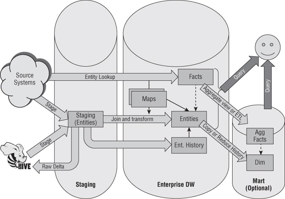
Figure 10.1 Visualizing Thomas Kejser's Big Picture Data Warehouse Architecture

Code First (Schema Later)

This code-first approach does have other advantages. Cleansing operations, for example, “get in the way” of mining the data for valuable nuggets of information. There is also reduced risk in using code first when you are keeping all the data in its raw form. You can always augment your program, redeploy, and restart the analysis because you still have all the data at your disposal in its raw form.

You can't always go back if you have observed a schema-first approach. If you have modeled the data to follow one structure you may have transformed or aggregated the source information making it impossible to go back to the beginning and reload from scratch. Worse still, the source data may have been thrown away, which could have been collected years ago, it might be difficult or in some cases impossible to get that data back.

Consequently, Hadoop developers tend to shy away from a schema-first/code-later design. They worry less about the structure of the data and instead focus on looking for the value in the data. Remember, Hadoop developers aren't so motivated by plugging gaps in a key performance indicator (KPI) report. Data scientists, especially, are looking for new insights, which is, by its very nature, a more experimental paradigm.

Model the Value

Once a valuable pattern has emerged, we have something we can apply a schema to. However, don't just constrain your thinking when you see the word model. In the world of analytics, that model may just be an algorithm that has identified some interesting trends or shapes in the data.

A Hadoop developer may choose to harden the solution at this point and also may “graduate” the results of the insights to a new Hadoop environment for users to consume. This pattern is surprisingly common. Don't assume that there is only one Hadoop cluster to support one production environment.

In Figure 10.2, you can see an example of what the Hadoop environment might look like and how the data could graduate between environments. The far-left bar represents the Bronze environment. This is the raw data and is an environment typically used by the “data scientist” mining for value. As patterns emerge and value is established, the results might find themselves moving into the Silver environment for “power users” or “information workers” to work with. There are usually more power users than there are data scientists. Finally, the data may go through one last graduation phase from Silver to Gold. This might be the environment exposed to the broadest spectrum of the business (that is, the “consumers” of the data). If there are dashboards to be built and so forth, it is likely that Gold is the target environment to perform these tasks.

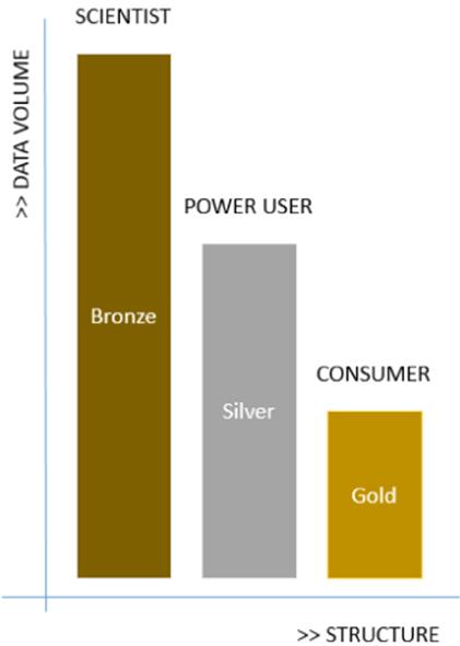
Figure 10.2 Understanding Gold, Silver, and Bronze Hadoop environments

As the data graduates, we should start seeing other patterns emerge. These patterns aren't constrained to the value in the data but also to attributes of the data. Typically, we'll see the data take on greater structure to facilitate more mainstream analysis and integration with other tools. Furthermore, we would expect to see improvements in data quality and integrity in these other environments. When we think about integrating this data with the broader enterprise, this becomes increasingly important (because we need to pick our moment when it comes to data integration).

Throw Compute at the Problem

All this flexibility comes at a cost, and that cost is a need to throw greater amounts of compute power at the problem. This philosophy is baked into Hadoop's architecture and is why batch engines like MapReduce exist. MapReduce's ability to scale compute resources is a central tenet of Hadoop. Therefore, Hadoop developers have really taken this to heart.

In some cases, there is an overreliance on this compute, which can lead to a level of laziness. Rather than optimize the data processing and possibly leverage other technologies, Hadoop developers can “waste” CPU by re-executing the same MapReduce program over and over. Once the trend has been established, the unknown unknown has been identified. It is now a known unknown.

Remember that the MapReduce program knows nothing about the data in the files contained within the Hadoop Distributed File System (HDFS). This is in stark contrast to the approach taken by relational database systems. The schema and model imposed by a database designer empowers the database engine to hold statistical information on the data held inside the tables. This leads to optimized computing and a significant reduction in compute resources required.

As Hadoop 2.0 takes hold, it will be interesting to see how the Hadoop community adopts other engines. We'll have to see how quickly they move to interactive query with Tez as the underpinning engine, for example. Furthermore, we'll have to wait and see which engine is adopted by the community for other types of problems. The battleground seems drawn for complex event processing, for example. Are you ready for the Flume versus Storm showdown? One thing is certain: how each project leverages the compute at its disposal will be a significant factor. It will, however, only be one factor. Expect ease of programmatic use to be just as important, if not more important. After all, the “winner” will be the project that offers the fastest “time to insight.” In the world of Hadoop, insight is king.

Introducing Parallel Data Warehouse (PDW)

Much like the SETI@Home program, Parallel Data Warehouse (PDW) is a scale-out solution, designed to bring massive computing resources to bear on a problem. Both PDW and SETI, therefore, are massively parallel processing (MPP) systems. However, unlike SETI, PDW is designed to support many forms of analysis, not just for searching for alien life.

PDW is a distributed database technology that supports set-based theory and the relational model. This is what sets it apart from Hadoop, even when used with Hive. PDW supports transactions, concurrency, security, and more. All the things you expect from a database, but backed by significantly more resources, courtesy of the scale-out architecture.

Currently, PDW can sometimes be seen by the market as being a niche technology. For starters, Microsoft is not ubiquitously known for building scale-out database technology products. It has one: PDW. It is known for building SQL Server, which is a scale-up solution. It is, therefore, not always at the forefront of architects' minds when building distributed systems. Furthermore, it's often perceived that MPP systems are expensive and, therefore, suitable only for truly massive datasets that are petabytes in size. This is not the way to think about MPP or PDW. MPP solutions aren't as expensive as people think. Likewise, scaling storage capacity is only one goal when using an appliance like PDW. However, it is the most easily understood aspect, and so this is why people talk about it most. I really think it is the least compelling reason.

Consequently, this general lack of brand awareness, coupled with some preconceived technology notions, often results in MPP technology and PDW being eliminated from a solution build before being investigated as an option. This is a real shame. I've seen many customers who would have really benefitted from PDW, but have chosen to implement on SMP technology and have suffered as a consequence. Even when they have heard of PDW, some people have ultimately reached for their security blanket and architected for SMP. I know some of those customers, and they are regretting that decision.

Therefore, in this section we are going to focus on the what, why, and how of PDW so you, the reader, get a much better understanding of why PDW is an important technology that delivers great value to business users. My intention is that you can also use this information to make an informed decision in your next project.

What Is PDW?

PDW is unlike any other technology in the Microsoft Data Platform. For starters, it is not just software, and it's more than hardware plus software. It's an appliance. That means it comes with both hardware and software all preconfigured to offer best practices, high availability, and balanced performance, thus reducing the burden on the developers and the operations team.

The analogy I like to use is that of a kettle. Kettle's do a job for you. They boil water. You could use a pan on the stove, but you don't. If you want to boil water quickly and easily, you buy a kettle. You might look online, read some reviews, and check pricing; but basically, you find one that performs to your needs (and preferably matches the décor of your kitchen). One quick trip to the store and you have a kettle. You unbox it, plug it in, and away you go. You are boiling water, quickly, simply, and efficiently. Remember, though, that it's an appliance. It has a specific purpose; you can't use a kettle to heat soup. (Well, you can, but the result is less than ideal.)

PDW is the same. You can do some research online, pick your preferred hardware vendor (HP, Dell, or Quanta), and decide how much compute resources you want to have at your disposal. You order the kit, and 4 to 6 weeks later a preinstalled, preconfigured rack arrives at your data center. It's unboxed (consider this a white glove service), plugged in, and plumbed into your network. Data warehousing in a box. Note that this is not transactional processing in a box. Remember, we support boiling water, not heating soup with PDW.

NOTE

Quanta have only recently entered the market. At the time of writing the PDW appliance using Quanta is only available in the USA and China. Both HP and Dell are available worldwide.

Okay, so the question that tends to follow is this: What happens if you want to boil water more quickly or boil greater quantities of water? You simply buy a bigger/better kettle. The same applies with PDW. If you want queries to run faster or you want to handle more data, you can simply extend your appliance to provide you with additional computing resources. The nice part of extending PDW is that the costs are known, predictable, and linear. This is one of the key aspects of scale-out solutions. When you extend them you are using more of the same commodity kit.

Contrast this with a normal SQL Server data warehouse build, even one with guidance like a Fast Track solution. These are more like buying a box of Lego. Sure, they come with instructions and guidance on assembly, but it's up to you to assemble it correctly. If you don't follow the instructions you are unlikely to have built the Lego Hogwarts castle you purchased. You are much more likely to have created something completely different. It might look like a castle and feel like a castle but it won't be Hogwarts. The same principle applies to Fast Track.

Furthermore, how do you extend it? Well, extending a server isn't really very simple, is it? It's not like you can graft another couple of CPU sockets onto the motherboard, now is it?

Why Is PDW Important?

PDW is actually branded SQL Server Parallel Data Warehouse. This leads to misconceptions about what PDW is or isn't. Actually, it'd be more accurate to say it is Parallel Data Warehouse, powered by SQL Server. There is an important but subtle difference. SQL Server is a mature utilitarian database engine with some enhanced functionality aimed at improving performance for the data warehouse workload. It has a myriad of features and options to support other workloads and products as well. PDW is different. PDW is designed purely for data warehousing. It is built as a black box solution that is designed to streamline development, improve performance, and reduce the burden on operational teams.

However, here is a different way of looking at PDW:

“PDW is the de facto storage engine for data warehousing on the Microsoft Data Platform.” — James Rowland-Jones, circa 2013

I realize that I am quoting myself. It's not my intention to be egotistical. However, I do believe it to be true, and I don't know of anyone else who has come out and publicly said anything to the same degree. Besides which, I want to share with you my reasoning. I don't know when I started using it exactly, but it is something that has resonated well with attendees of the PDW training I've given, and I hope that it will resonate with you too.

To help back up my somewhat grandiose hypothesis, I want to draw your attention to the following key points, which I explain more fully in the following sections:

· PDW is the only scale-out relational database technology in the Microsoft Data Platform.

· Data warehouse features come first to PDW.

· PDW is the only Microsoft relational database technology that seamlessly integrates with Hadoop.

· PDW has two functional releases a year.

PDW Is the Only Scale-out Relational Database in the Microsoft Platform

Some attempts have been made at scale-out with the likes of federated databases and distributed partitioned views, but it is also fair to say that SQL Server was designed to scale up. It was also not designed from the ground up with data warehousing in mind. PDW, however, is designed in this way. It is a workload-specific appliance focused on the data warehouse.

The fact that PDW is a scale-out technology is incredibly important. It places Microsoft into the same bracket as other vendors of MPP distributed databases, such as Teradata, Netezza, Oracle, SAP HANA, and Pivotal, with technology that has the ability to scale to the demands of big data projects. The only relational database technology that has any presence in the world of big data involves scale-out MPP databases. Each and every one of them purports to have integration with Hadoop in some form or other. PDW is no exception.

MPP databases offer some compelling benefits for the data warehouse and for big data. The primary benefit is the ability to scale across servers enabling a divide and conquer philosophy to data processing. By leveraging a number of servers, PDW can address many more CPU cores than would ever be possible in an SMP configuration.

In its biggest configuration, PDW supports 56 data processing servers (known as compute nodes) comprising the following resources:

· 896 physical CPU cores

· 14TB of memory

· 6PB+ of storage capacity

What is even more impressive is that PDW forces you to use all these resources. In other words, it forces parallelism into your queries. This is fantastic for data warehousing.

Imagine having an option in SQL Server that gave you an option to run with a minimum degree of parallelism or MINDOP(448). You can't? No, of course you can't, because there is no such option in SQL Server. With PDW, you have that by default.

Understanding MINDOP

448 represents one thread for every distribution on a 56–compute node appliance. There are 8 distributions on each node. In this configuration PDW would issue 448 separate queries in parallel against a distributed table. Hence, MINDOP(448). Fear not, we will discuss distributions and distributed tables shortly. The key takeaway here is that PDW delivers an additional level of parallelism that simply isn't available in SQL Server.

Data Warehouse Features Come First to PDW

Just think about this list of features; all were first in PDW:

· Updateable column store

· Enhanced batch mode for query processing

· Native integration with Hadoop via Polybase

· New Cardinality Estimator

· Cost-based Distributed SQL Query Engine

· New windowing functions including lag and lead

It's a pretty impressive list. I am sure that there are other examples, as well. In the case of Polybase, it is an exclusive feature, as well, which helps to define PDW's unique selling point (USP).

PDW and Hadoop

We just touched on this, and it is worth restating. PDW offers native integration with Hadoop via Polybase—something that we are going to really dive into later in this chapter. The key takeaway here is that Polybase is integrated into a component of PDW, not a component of SQL Server. That component is called the Data Movement Service (DMS).

NOTE

The fact that the DMS was chosen as the integration point means that this feature isn't coming to the box product known as SQL Server anytime soon. The DMS is PDW specific, so if you want to get on the Polybase bus, you will need to buy a PDW ticket.

PDW Release Cadence

As mentioned previously a few times now, PDW is an appliance, an integrated blend of both hardware and software. This fact has other implications that are less obvious. For example, PDW doesn't do service packs. PDW has appliance updates (AUs), with the team committed to delivering an AU every 6 months.

AUs differ from service packs in one notable way. The releases are functional and do not just contain fixes to defects. In actual fact, they are packed full of features targeting the data warehouse work stream. Therefore, the team can rev the product in a much more agile fashion and respond to customer demand as appropriate.

How PDW Works

We are going to start by keeping things simple and build from there. This section is a conceptual introduction to PDW.

PDW uses a single master node known as the control node as the front door to the appliance and is the gateway to the data. The data is held on a number of compute nodes. The vast majority of data processing occurs in the compute nodes. The ability to continually add compute nodes gives PDW its scale-out ability. The challenge when scaling out is that different subsets of data are held on different nodes and may need to seamlessly move the data to resolve a users' query. PDW achieves this with an external process called the Data Movement Service (DMS).

NOTE

The DMS is not part of SQL Server; it is an entirely separate process. When data needs to move across the appliance, DMS moves it. The DMS exists on both the control and the compute nodes and is managed by its own DMS Manager that resides on the control node.

The compute and control nodes are connected together by two networks: Ethernet and Infiniband. The Ethernet network manages basic communication between the nodes: heartbeat, status, acknowledgments, that sort of thing. The Infiniband network is used for moving data. Infiniband is an ultra-low-latency network, which is ideally suited for moving large volumes of data at speed. PDW uses FDR Infiniband, which is capable of sustaining 56Gbps.

When you connect your application, including SQL Server Data Tools (SSDT), you will connect to the control node. The control node accepts the request, generates the DSQL plan and orchestrates a series of highly parallelized operations across the compute nodes, thus achieving scale out. However, the real secret to how PDW works is down to how it creates databases and tables.

Distributed Databases

Think about a piece of toast. That piece of toast is your PDW appliance. Now what do you want to put on that toast? Butter and Marmite, of course!

I LOVE Marmite

For the international audience who might not understand the reference Marmite is a vegetarian savoury spread made from yeast extract that is itself a by-product of brewing beer. Please head over to https://www.facebook.com/Marmite for more details. Better still go and try it! Unless you are in Denmark, of course, where it is banned—only the Danes really understand why. Too bad; I know many of them love it there, too.

Now when spreading butter on your toast, you want to make sure that you get a nice even spread across the slice. Marmite has quite a strong, distinctive flavor, so it's even more important that you get this right. You want to make sure that every bite you take gets a bit of everything; not too much to be overbearing, and not too little so you can't taste it. You want it even. The same applies to PDW. The need to keep things even starts with the database creation:

CREATE DATABASE AdventureworksPDW2012

WITH

(

REPLICATED_SIZE = nn

, DISTRIBUTED_SIZE = nn

, LOG_SIZE = nn

, AUTOGROW = ON | OFF

)

That is it! PDW handles the rest. PDW takes this information and converts this into data definition language (DDL) that it can use to drive parallelism in the appliance. Let's look at what CREATE DATABASE does and then each of these properties in turn.

Create Database

Although only one CREATE DATABASE statement is fired, as shown in the preceding code, many are created. One database is created on each compute node, and one database is created on the control node. What is important to understand is that their purposes differ significantly.

The database created on the control node is there to hold the metadata about the database. This database is also referred to as the shell database. Apart from holding all the security configuration, table, and procedure definitions, it also holds all the consolidated statistics from all the other databases held on the compute nodes. The shell database is actually very small; it holds no user data. Its primary function is during query optimization. There's more to come on that topic later in this chapter.

WARNING

Directly Accessing PDW's SQL Servers and the Shell Database PDW does not let you directly access the SQL Servers either on the control node or the compute nodes. This is to ensure that no inadvertent changes are made that could damage PDW and potentially void the warranty. Consequently, whilst it is an important component to understand, the shell database is not directly accessible by end users. It's created purely for PDW to use.

Each compute node also has a database created. These databases are where all the user data is stored. These databases have a rather interesting configuration. They consist of 10 separate filegroups that are key to PDW's parallelism. Each database on each compute node has all 10 filegroups. I've detailed them in the all in the matrix shown in Figure 10.3.

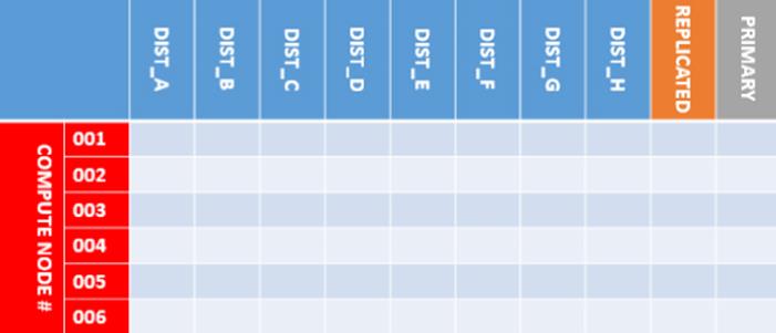
Figure 10.3 The bucket matrix created by PDW for holding user data

I have listed out all the filegroups on the x-axis of the matrix and shown compute nodes on the y-axis. This symbolizes something important. Every compute node has its own database each with their own set of filegroups. The matrix represents the total number ofbuckets available to PDW for depositing data. This really is the key to how PDW works. The more compute nodes you have, the more buckets.

The filegroups on the x-axis start with some unusually named ones DIST_A - DIST_H. These are called distributions and are designed for a certain type of table called a distributed table. The next filegroup is called replicated. You will notice that there is only one of these. That is significant. This filegroup holds replicated tables.

Don't worry if all this talk of different table types is a bit confusing; we are going to talk about distributed and replicated tables later in this chapter. Suffice it to say that PDW supports two types of tables: distributed and replicated. When creating a table, we decide whether we want to distribute the data across the appliance (in which case we use a distributed table) or if we want to replicate the table. Typically, large facts are distributed, and dimensions are replicated. This is not always true, but it is a reasonable starting point.

For completeness, we need to recognize the primary filegroup. The primary filegroup only holds data system table metadata for your database objects just like a regular SQL Server database. The only difference is that we do not let user data go into the primary filegroup. Most of the time, we ignore that it is even there.

You should now see that the CREATE DATABASE statement is logical; that is, it is used to create multiple physical databases to support the one database you have specified. To help facilitate this shift from logical to physical, PDW implements a layer of abstraction. An example of that can be seen with the database name. Only the database built on the control node would be given the name you have specified. The databases on the compute nodes have a different name. It follows the convention of DB_ followed by 32 alphanumeric characters. This abstracted name is used on every compute node. PDW exposes this mapping via a PDW-specific catalog mapping view called sys.pdw_database_mappings. Here is some sample code and the results (See Figure 10.4):

SELECT d.name

, dm.physical_name

FROM sys.databases d

JOIN sys.pdw_database_mappings dm ON d.database_id = dm.database_id

WHERE d.name = 'AdventureWorksPDW2012'

Figure 10.4 Logical and physical database names in PDW

Replicated_Size

In Figure 10.4, you can see that we have six compute nodes and one replicated file group per compute node. The replicated size option allows you to size how big each replicated filegroup will be on each compute node. This value is measured in gigabytes (GB) and can be expressed as a decimal. Therefore, a replicated size of 10 will allocate 10GB on each compute node to the replicated filegroup.

Whatever value we specify for the replicated size, this is the value that will be used for all six replicated filegroups. There is no option to have different sizes. Data held in a replicated table is, in effect, a copy on every compute node, which is why the amount actually allocated is multiplied by the number of nodes you have. In reality, when specifying replicated size, you simply need to decide how much capacity you need to hold all the data once. PDW actually takes care of the actual allocation and the replication of the table. The fact that we will be holding it six times is really an internal optimization.

The replicated filegroup is only used by PDW when we decide to create a table and specify that we wish to replicate it. Because these tables tend to be our dimensions, we typically expect to see a relatively small size allocated here. If someone had allocated terabytes rather than gigabytes, that would warrant serious investigation.

Distributed_Size

The distributed size value is used differently from the replicated size. The distributed size value provided in the CREATE DATABASE statement is actually evenly split across all the distributions to ensure we have the same space available in each bucket for distributed data. Data is then spread across the distributions with each distribution holding a distinct subset of the distributed table data. Again, the value supplied in the DDL statement is also measured in gigabytes and can be expressed as a decimal.

If you remember back to the toast analogy, we also want to spread it as evenly as possible over the appliance. Therefore, if we have 6 compute nodes in our PDW appliance, we also have a total of 48 distributions (8 distributions per node A-H). If I allocate 10TB as my distributed size, I am therefore allocating 1/48 of this to each distribution. In this example, each distribution would be allocated approximately 213.33GB of the available capacity. However, I would have allocated 10TB in total, which I would use for my distributed tables.

Remember, the distributed size is used only by tables that have been specified as distributed. These are likely to be fact tables; so don't be surprised to see a very large number here, a very significant percentage of the total allocated. Furthermore, there is no replication of data in a distributed table. This sets distributed tables apart from replicated tables. In reality, both types of tables rely on disk RAID configurations for data protection.

Log_Size

The log size value behaves similarly to the distributed size, in as much as it is spread evenly across the appliance. Therefore, if I have 6 compute nodes and a 10GB log file, I will split my log file allocation into 6 approximately 1.6GB allocations. Remember that SQL Server doesn't create a filegroup for the log files.

In actual fact, the log file is split further again. PDW doesn't create just one log file for the database. It creates one log file per disk volume instead. With the HP AppSystem for PDW, for example, there are a total of 16 volumes per compute node. Therefore, a 10GB log_size specification for our 6 compute nodes would actually result in 96 log files, with each one being approximately 106.6MB in size. By doing this kind of allocation, PDW ensures that the log file grows evenly across all its available storage and isn't constrained to a single volume. Furthermore, each volume soaks up some of the load from the database log. Typically, the log will be double the size of the largest (uncompressed) file loaded.

Autogrow

PDW will run an autogrow on the database files rather than fail a query that asks for additional capacity when the files are full. In PDW, the autogrow option affects only the databases created on the compute nodes. This is important because PDW's metadata via sys.database_files is a bit misleading. This catalog view shows the information for the shell database held on the control node, not the actual values set against the compute node.

Table 10.2 and Table 10.3 show the actual values set against the compute node.

Table 10.2 Autogrow Settings for Compute Node Database Files (Excluding the Primary Filegroup Data Files)

Table 10.3 Primary Filegroup Autogrow Settings for Compute Node Database Files

With this information, we can see that PDW handles the data file in the primary filegroup differently from all other files and filegroups. In short, the primary always grows irrespective of the CREATE DATABASE setting for AUTOGROW. This makes sense; it's not something we've actually specified in the DDL, and the space consumed is tiny. We certainly wouldn't want a DDL request such as CREATE TABLE to fail for lack of storage. I have included this here just for completeness of information.

More important is that the other database files and log files are handled differently. Furthermore, these allocations are fixed by the release and do not change (at the time of this writing) based on size of the database; that is, it does not matter whether your database is 1TB or 1PB, the AUTOGROW value is the same. It also doesn't matter whether the filegroup is for distributed or replicated tables, the autogrow works in exactly the same way.

Finally, it should also be clear that PDW is not simply offering up SQL Server functionality. AUTOGROW in PDW is very different than AUTOGROW in SQL Server. Each filegroup type has been evaluated for the AUTOGROW function, and a predesigned, tested configuration is applied on your behalf. This is classic appliance behavior.

Therefore, in conclusion, the AUTOGROW function is really there to prevent failures and 3:00-a.m. alarm support calls! We should definitely be monitoring for consumption of our pre-sized database and log files and be proactive with our management of storage capacity. You can consider it a good practice to preallocate your distributed, replicated, and log sizes for your anticipated growth. A typical projection would be roughly six months to a year. That gives you enough space to fine-tune future allocations without over-allocating in the first instance.

Distributed Tables

Distributed tables are the heart of PDW and are key to understanding its parallelism. In PDW, a table is defined as being distributed when it is created. We pick a column (yes, only one, just like partitioning) and hash the distinct values of this column, allocating each distinct value into one of our buckets. To be a bit more precise, the hash is performed by the DMS as the data is written to the table. Let's look at an example:

CREATE TABLE [dbo].[FactInternetSales]

(

[ProductKey] int NOT NULL,

[OrderDateKey] int NOT NULL,

[DueDateKey] int NOT NULL,

[ShipDateKey] int NOT NULL,

[CustomerKey] int NOT NULL,

[PromotionKey] int NOT NULL,

[CurrencyKey] int NOT NULL,

[SalesTerritoryKey] int NOT NULL,

[SalesOrderNumber] nvarchar(20) NOT NULL,

[SalesOrderLineNumber] tinyint NOT NULL,

[RevisionNumber] tinyint NOT NULL,

[OrderQuantity] smallint NOT NULL,

[UnitPrice] money NOT NULL,

[ExtendedAmount] money NOT NULL,

[UnitPriceDiscountPct] float NOT NULL,

[DiscountAmount] float NOT NULL,

[ProductStandardCost] money NOT NULL,

[TotalProductCost] money NOT NULL,

[SalesAmount] money NOT NULL,

[TaxAmt] money NOT NULL,

[Freight] money NOT NULL,

[CarrierTrackingNumber] nvarchar(25) NULL,

[CustomerPONumber] nvarchar(25) NULL

)

WITH

( CLUSTERED COLUMNSTORE INDEX

, DISTRIBUTION = HASH([SalesOrderNumber])

, PARTITION

(

[OrderDateKey]

RANGE RIGHT FOR VALUES

(

20000101

, 20010101

, 20020101

)

)

);

In the preceding code listing you can see that a lot is familiar to you. However, you can see I have highlighted the key difference: DISTRIBUTION = HASH([SalesOrderNumber]). This means that every SalesOrderNumber will be hashed and allocated to one of our buckets. It is therefore essential that we pick a value with a good number of distinct values (my rule of thumb is 1000) to make sure the data is spread evenly across the appliance and avoids something we call data skew.

There is actually one consideration that would take precedence over the data skew rule. When large fact tables are joined together (i.e., with a fact-to-fact join), we can often see significant volumes of data being moved across the appliance. This occurs when the two facts are not distributed on the same column. In these situations it is vital that we try to prevent the DMS from moving data to resolve the join. We can achieve this by distributing both fact tables on the same column, ensuring that this column is also used in the join—even if the column is not absolutely required to satisfy the join criteria. The presence of a shared distribution key in the join will prevent a DMS movement of data, which will have a positively dramatic impact on performance. When faced with the prospect of large fact-to-fact joins, data skew is a secondary consideration.

You might be wondering why this table doesn't specify which filegroup it is on. It's a great question. Well, the answer is simply that this table definition doesn't really exist on the compute nodes. PDW does create this table on the control node inside the shell database, though, as you might have suspected. However, after that, PDW has to manage creating one copy of this table for every distribution. Because we have eight distributions per compute node, we need eight different names for this table. The naming convention is similar to the one used for databases TABLE_32AlphanumerChars_[A-H]. You can see these table mappings via the sys.pdw_table_mappings view:

select t.name

, ptm.physical_name

from sys.tables t

join sys.pdw_table_mappings ptm on t.object_id = ptm.object_id

where t.name = 'FactInternetSales'

Figure 10.5 shows the result.

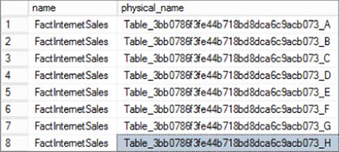
Figure 10.5 Comparing logical and physical table names in PDW

As for understanding which column was the one we distributed on, we need a different query. This information is not held on sys.columns, and so we need to look into some PDW proprietary extensions for this information:

SELECT t.name AS TableName

, tp.distribution_policy_desc AS TableDistributionPolicyDesc

, c.name AS ColumnName

, y.name AS DataType

, c.max_length AS DataMaxLength

, c.precision AS DataPrecision

, c.Scale AS DataScale

, c.collation_name AS ColumnCollation

, c.Is_Nullable AS ColumnIsNullable

, cm.distribution_ordinal AS IsDistributionColumn

FROM sys.columns c

JOIN sys.pdw_column_distribution_properties cm

ON c.object_id = cm.object_id

AND c.column_id = cm.column_id

JOIN sys.types y ON c.user_type_id = y.user_type_id

JOIN sys.Tables t ON c.object_id = t.object_id

JOIN sys.pdw_table_distribution_properties tp

ON t.object_id = tp.object_id

The abridged results for this query are shown in Figure 10.6. Notice that the TableDistributionPolicyDesc column states HASH as it is a distributed table and that the SalesOrderNumber row has a 1 for the IsDistributionColumn.

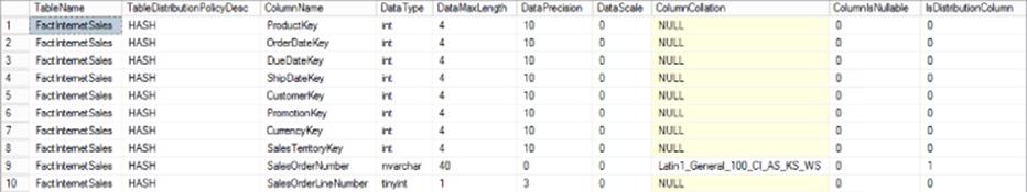
Figure 10.6 Extended table and column properties for distributed tables

This query works just as well for showing off additional data about replicated tables too. Let's look at them now.

Replicated Tables

Replicated tables tend to be smaller tables, typically dimensions, which represent whole copies of data. A replicated table has its entire data set copied to all the compute nodes. Why do this? Well, it really helps when reading the data. At the end of the day, each compute node is a highly tuned SQL Server SMP instance with one buffer pool of memory. To facilitate a join, PDW needs to ensure that all the data is available. By replicating a table, we guarantee that this table at least has all its data available for a local, co-located join.

However, if the join was between two distributed tables, we may have an issue. It's still possible, of course, that both tables may be distributed in the same way; this is often a primary design goal. However, it's not always possible. Under some circumstances, one of the tables may have to be redistributed to make the join compatible. The worst case is realized when either table is distributed on a joining key. In this case both tables need to be redistributed. This is called a double shuffle.

It is important to note that data movement can even happen with a replicated table. When the join is an outer join, this triggers movement because we have to handle the nulls generated by the join.

This is quite an advanced topic, and so we aren't going to be able to cover it here. However, suffice to say that by replicating small dimension tables and inner-joining them to our distribution table, we avert the need to redistribute data because of the join. However, hopefully you can see that we need to pay careful attention to our table design, as it can have a dramatic impact on performance.

Naturally, there is a price to pay for this read enhancement. That price is in the form of delayed writes. Consider for a moment our six-compute-node deployment of PDW. If we have a replicated table, we will need to write the same row six times to ensure consistency. Writes to replicated tables are therefore much slower than to distributed tables. You can imagine that if a user were able to read the data partway through this write that the user would end up with inconsistent results. Therefore, the write is also a blocking transaction.

Under normal operation, these are good trade-offs. The write penalty is a one-time-only operation, and hopefully we can batch these up to maximize efficiency.

Finally, PDW also performs the same abstraction for table names of replicated tables as it does for distributed ones. A slight difference exists, though, inasmuch as we need to create only one mapping name, and so the naming convention differs slightly. For replicated tables, it is TABLE_32AlphanumericCharacters. To see the value created, we can use the sys.pdw_table_mappings catalog view as before.

Hopefully, you now have an appreciation for the what, why, and how of PDW and are intrigued enough to consider it in your environment. In this next section, we are going to talk about the one feature that's completely unique to PDW—its jewel in the crown, Project Polybase.

Project Polybase

Project Polybase was devised by the Gray Systems Lab (http://gsl.azurewebsites.net/) at the University of Wisconsin–Madison, which is managed by Technical Fellow Dr. David DeWitt. In fact, Dr. DeWitt was also instrumental in the development of Polybase, and is himself an expert in distributed database technology.

The goal for Polybase was simple: provide T-SQL over Hadoop, a single pane of glass for analysts and developers to interact with data residing in HDFS and to use that “nonrelational” data in conjunction with the relational data in conventional tables.

The goal was simple, but the solution was not. It was so big that Polybase had to be broken down into phases.

We've talked about Polybase and Hadoop integration a few times in this chapter. This section dives right into it:

· Polybase architecture

· Business use cases for Polybase today

· The future for Polybase

Polybase Architecture

Polybase is unique to PDW. It is integrated within the PDW's DMS. The DMS isn't shipped with any other SQL Server family product. Therefore, I think it's fair to claim Polybase for PDW.

Polybase extends the DMS by including an HDFS Bridge component into its architecture. The HDFS Bridge abstracts the complexity of Hadoop away from PDW and allows the DMS to reuse its existing functionality; namely, data type conversion (to ODBC types), generating the hash for data distribution and loading data into the SMP SQL Servers on residing compute nodes.

This section details the following:

· HDFS Bridge

· Imposing structure with external tables

· Querying across relational and nonrelational data

· Importing data

· Exporting data

HDFS Bridge

The HDFS Bridge is an extension of the DMS. Consequently, it is a unique feature to PDW. Its job is to abstract away the complexity of Hadoop and isolate it from the rest of PDW while providing the gateway to data residing in HDFS. Remember that the world of Hadoop is a Java-based world, and somewhat unsurprisingly PDW is C# based.

The HDFS Bridge then uses Java to provide the native integration with Hadoop. This layer is responsible for communication with the NameNode and for identifying the range of bytes to read from or write into HDFS residing on the data nodes. The next layer up in the HDFS Bridge stack is a Java Native Interface (JNI), which provides managed C# to the rest of the DMS and to the PDW Engine Service.

In Figure 10.7, you can see that the HDFS uses the Java RecordReader or RecordWriter interface to access the data in Hadoop. The RecordReader/Writer is a pluggable element, which is what allows PDW to support different HDFS file types.

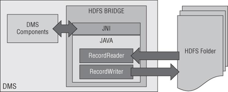
Figure 10.7 HDFS bridge architecture and data flow

Polybase gets much of its power through its ability to parallelize data transfer between the compute nodes of PDW and the data nodes of HDFS. What is interesting about this is that Polybase achieves this transfer with runtime-only execution information.

The PDW Engine uses the HDFS Bridge to speak with the NameNode when handed a Polybase query. The information it receives is used to divide the work up among the compute nodes as evenly as possible. The work is apportioned, with 256KB buffers allocated to stream rows back to the DMS on each compute node. The DMS continues to ingest these buffers from the RecordReader interface until the file has been read.

Imposing Structure with External Tables

PDW uses a DDL concept called an external table to impose the structure we require on the data held in the files of HDFS. The external table is really more akin to a BCP format file or a view than it is a table. (We will look at the internal implementation of external tables shortly.)

It is important to note that the coupling between PDW and Hadoop is very, very loose. The external table merely defines the interface for data transmission; it does not contain any data itself nor does it bind itself to the data in Hadoop. Changes to the structure of the data residing in Hadoop is possible, and even the complete removal of the data is conceivable; PDW would be none the wiser. In tech speak, unlike database views there is no schema-binding option available here. We cannot prevent a table from disappearing in Hadoop by creating an external table. Likewise, when we delete an external table, we do not delete the data from HDFS.

Furthermore, there are no additional concurrency controls or isolation levels in operation either when accessing data through an external table. While there is schema validation against the existing external table object definitions, it is quite possible you may see a runtime error when using Polybase. However, this is part of the design and helps Polybase retain its agnostic approach to Hadoop integration.

External tables are exposed via the sys.external_tables catalog view and in the SSDT tree control. The view inherits from sys.objects, and it exposes to us all the configuration and connection metadata for the external table.

Following is an example of an external table. Imagine if you will that the data for the AdventureWorks table FactInternetSales existed in HDFS. We are still bound by the restriction of having unique names for objects in the same database, so for clarity I have named data residing in Hadoop with an HDFS prefix:

CREATE EXTERNAL TABLE [dbo].[HDFS_FactInternetSales]

(

[ProductKey] int NOT NULL,

[OrderDateKey] int NOT NULL,

[DueDateKey] int NOT NULL,

[ShipDateKey] int NOT NULL,

[CustomerKey] int NOT NULL,

[PromotionKey] int NOT NULL,

[CurrencyKey] int NOT NULL,

[SalesTerritoryKey] int NOT NULL,

[SalesOrderNumber] nvarchar(20) NOT NULL,

[SalesOrderLineNumber] tinyint NOT NULL,

[RevisionNumber] tinyint NOT NULL,

[OrderQuantity] smallint NOT NULL,

[UnitPrice] money NOT NULL,

[ExtendedAmount] money NOT NULL,

[UnitPriceDiscountPct] float NOT NULL,

[DiscountAmount] float NOT NULL,

[ProductStandardCost] money NOT NULL,

[TotalProductCost] money NOT NULL,

[SalesAmount] money NOT NULL,

[TaxAmt] money NOT NULL,

[Freight] money NOT NULL,

[CarrierTrackingNumber] nvarchar(25) NULL,

[CustomerPONumber] nvarchar(25) NULL

)

WITH

( LOCATION='hdfs://102.16.250.100:5000/files/HDFS_FactInternetSales'

, FORMAT_OPTIONS

(

FIELD_TERMINATOR = '|'

, STRING_DELIMITER = ''

, DATE_FORMAT = ''

, REJECT_TYPE = VALUE

, REJECT_VALUE = 0

, USE_TYPE_DEFAULT = False

)

);

Looking at the preceding code, you can see that it is indeed more like a BCP format file than anything else. In addition to the column names, types, and null-ability, we can also identify the location of both the cluster and the folder in HDFS holding the data, any field and row terminators, formatting for dates, both the method and the threshold for rejected records, and we can see how PDW should handle missing values when importing data using the USE_TYPE_DEFAULT option.

It is important to note, however, that although it doesn't really behave like one, an external table is actually a physical table. However, it is not created in Hadoop, nor is it present on the compute nodes like a normal table would be. It is instead created in the shell database up on the control node. You can see this by looking at the dsql query plan commands executed by PDW when we create an external table. In Figure 10.8, you can see the table is indeed created and that the location specifies it as the control node.

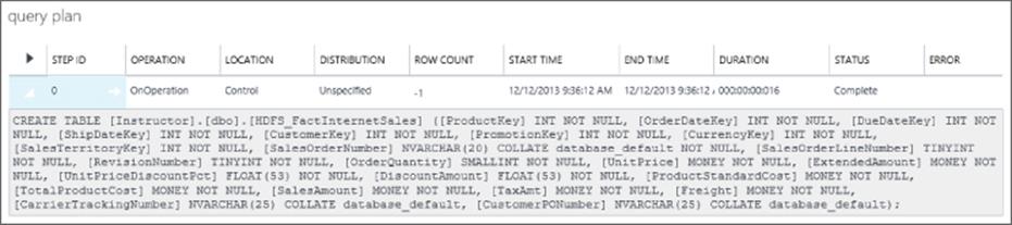
Figure 10.8 Creating the external table on the control node

As you can see, it is simply a normal table. However, this table is used only to hold statistics and metadata about the table. PDW does not allow any user data to be persisted in the control node. This includes external tables. The metadata includes all the properties we set at creation time of the external table itself. PDW attaches these metadata attributes using the sp_addextendedproperty system stored procedure, as shown in Figure 10.9.

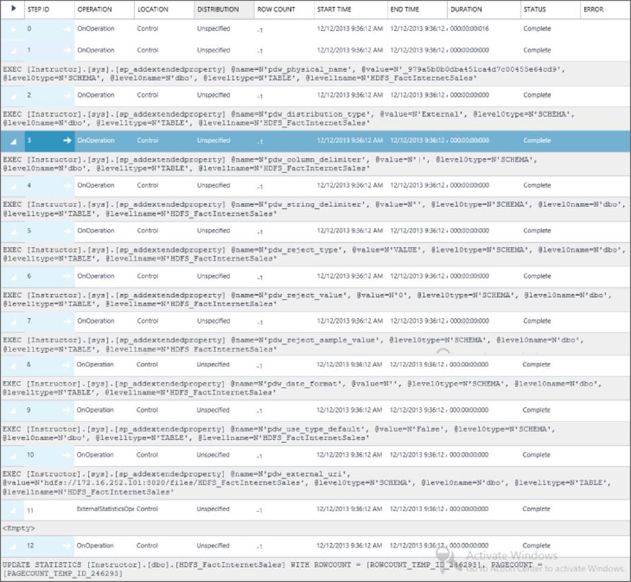
Figure 10.9 PDWs external table extended properties

The figure clearly shows all the metadata attributes you saw earlier in the DDL, as explained more fully in Table 10.4. A more useful location to see all this data is in the sys.external_tables catalog view.

Table 10.4 External Table Extended Properties

Figure 10.9 contains two other steps that are interesting:

· Step 11 - ExternalStatisticsOperation

· Step 12 - OnOperation

Although step 11 is “empty” (effectively hiding an internal operation), we can infer what action the external statistics operation is performing by looking at step 12. I've copied the code here:

UPDATE STATISTICS [Instructor].[dbo].[HDFS_FactInternetSales]

WITH ROWCOUNT = [ROWCOUNT_TEMP_ID_246293]

, PAGECOUNT = [PAGECOUNT_TEMP_ID_246293]

Clearly, then, PDW is retrieving what statistical data it can from Hadoop to determine the row length, number of rows in a process known as file binding. The file blocks are then allocated across the compute nodes as evenly as possible, for which we need to know the size of the table. This is called the split generation. This step is clearly the first in a long series of optimizations for the future phases of Polybase. Knowing the table size and knowing the row count are important first steps to cost-based optimization on Hadoop data.

Querying Across Relational and Nonrelational Data

“A single pane of glass,” that's what Polybase offers the business user—the ability to write a single query that analyzes data across both the relational data warehouse and the nonrelational data held in Hadoop. In that sense, Polybase is a uniter of worlds. Another way of looking at it is that Polybase is like a cow; it has many stomachs to digest data.

By leveraging the existence and structure of the external tables PDW is able to simply write queries against data residing in HDFS.

Consider this simple example (see Figure 10.10):

SELECT *

FROM dbo.HDFS_FactInternetSales FIS

OPTION

( LABEL = 'Polybase Read : Q001 : HDFS_FactInternetSales'

)

;

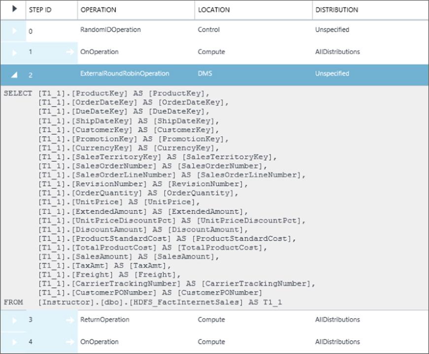
Figure 10.10 Simple Polybase query against data held in Hadoop

PDW is able to use the external table HDFS_FactInternetSales to read through to Hadoop and import the data residing in HDFS using a DMS operation called an ExternalRoundRobinOperation. This operation imports the buffers as is and simply allocates them on a round-robin basis to the compute nodes. As we do not need to join this table to any others, there is no need for anything more complex. Once allocated, the buffer is simply bulk inserted into a temporary table where it can be easily read by the ReturnOperation as shown in step 3 of the plan. The results are then streamed back to the client that issued the original query.

PDW can also initiate joins and aggregations between data held in one of its tables and data held in HDFS. In the following example, PDW is able to read data in HDFS through the same external table HDFS_FactInternetSales and subsequently join it to a number of tables in PDW (see Figure 10.11):

SELECT [EnglishProductCategoryName]

, [EnglishMonthName]

, SUM([TotalProductCost]) AS TotalCost

, SUM([SalesAmount]) AS TotalSales

FROM dbo.HDFS_FactInternetSales FIS

JOIN dbo.DimCustomer DC

ON FIS.CustomerKey = DC.CustomerKey

JOIN dbo.DimDate DD

ON FIS.[OrderDateKey] = DD.[DateKey]

JOIN dbo.DimProduct DP

ON FIS.[ProductKey] = DP.[ProductKey]

JOIN dbo.DimProductSubcategory DPS

ON DP.[ProductSubcategoryKey] = DPS.[ProductSubcategoryKey]

JOIN [dbo].[DimProductCategory] DPC

ON DPS.[ProductCategoryKey] = DPC.[ProductCategoryKey]

GROUP BY [EnglishProductCategoryName]

, [EnglishMonthName]

ORDER BY [TotalSales] DESC

, [EnglishProductCategoryName]

OPTION

( HASH JOIN

, LABEL = 'Polybase Read : Q002 : HDFS_FactInternetSales'

)

;

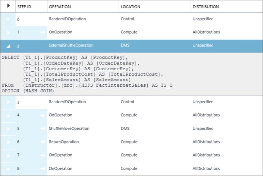
Figure 10.11 More complex Polybase query against PDW and Hadoop data

If you look at Figure 10.11, you will notice that this changes the plan and PDW uses a different DMS operation to source the data. Instead of the ExternalRoundRobinMove PDW uses the ExternalShuffleOperation. We require this operation as we are going to be performing joins. We will look at this new operation in more detail next as we investigate how PDW imports the data into its environment. It should hopefully be apparent that even when PDW is only reading data from the query perspective, it is, in fact, importing data first into PDW and then selecting from that imported data set. It therefore makes sense to look at the ExternalShuffleOperation more from both the query and import perspectives to understand the difference in the respective plans.

Importing Data with CTAS

PDW enables the parallel import of data through its CREATE TABLE AS SELECT (CTAS) statement. This is akin to a SELECT INTO in an SMP environment, but you have some added flexibility in terms of table geometry (distributed or replicated) and indexing.

To import data from HDFS, all you need to do is reference an external table in the SELECT part of the CTAS statement. This external table could have been created when the data was originally exported or simply could have been created over existing HDFS data. Either way, you simply reference the external table just like you would any other table. Following is a simple example:

CREATE TABLE dbo.FactInternetSales_Import

WITH (DISTRIBUTION = HASH([SalesOrderNumber]))

AS SELECT *

FROM HDFS_FactInternetSales fis

JOIN DimCustomer cus ON fis.CustomerKey = cus.CustomerKey

;

To facilitate the move from HDFS, the DMS has introduced a new movement type: the ExternalShuffleOperation. This movement selects the data “through” the external table (which provides PDW with the metadata required to access the data from HDFS) and shuffles the data using the DMS hashing function, distributing the data according to the hash (see Figure 10.12); first loading the data into a temp table, known as a Q table and then Inserting that data into the target user table.

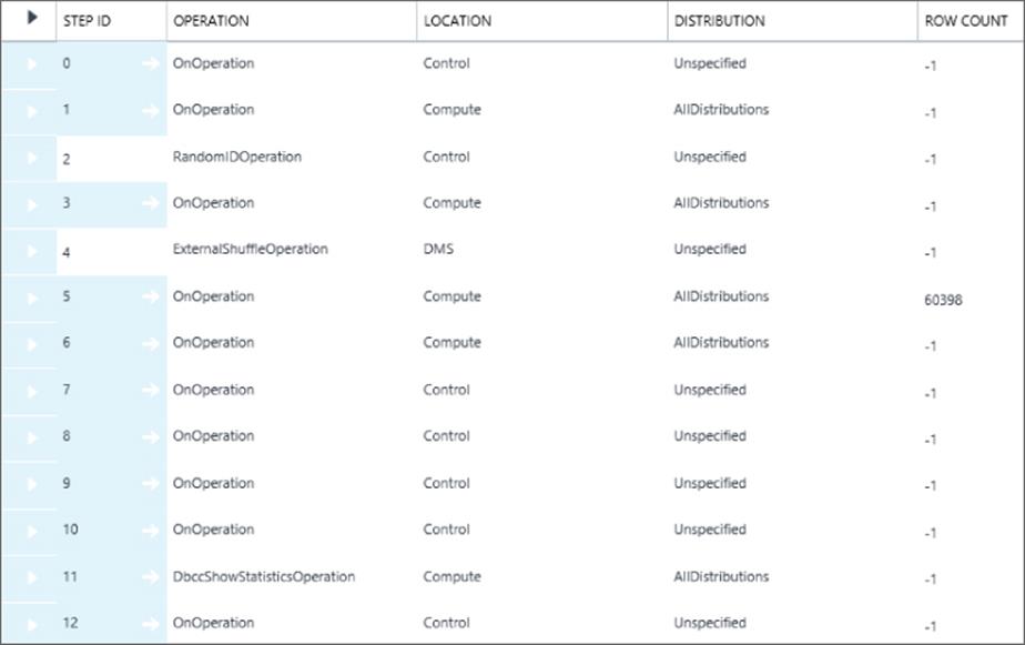
Figure 10.12 Importing data using the DMS and its ExternalShuffleOperation

The only difference between a query that performs a join and an import at this stage is that the import takes an additional step. An import persists the data in a user-defined table residing in a user database. In contrast, when running a Polybase query, PDW will still issue the DMS operation ExternalShuffleOperation but will instead only bulk-insert the data into a temporary table, in tempdb. PDW will then use that temporary table to satisfy joins and where-predicates to answer the user query.

We can see this clearly when we compare plans. If we look at the plan in Figure 10.9, we can see that there are a total of 13 steps. Step 5 is responsible for the insert of the rows into the table FactInternetSales_Import. The row count of 60,398 against step 5 is a telltale sign that this OnOperation is performing the insert. If we were to drill in, we'd have seen that the query was a select against the temp table with a MAXDOP 1 option applied to ensure a nice, clean, contiguous write into our target. Contrast this with Figure 10.11 andFigure 10.12. Neither query has an OnOperation immediately after their DMS operation. Both have moved on to perform other steps to fully resolve their queries. For the simple read, all that is left to do is to perform the ReturnOperation, which streams the results back to the client. Our more complex query needs to perform an aggregation that is not distribution compatible (we do not see the distribution key in the group by); therefore, it has to shuffle the data again before moving to its ReturnOperation.

However, if we look at the read query plan steps immediately preceding their respective Hadoop DMS operations, we can see that both read queries perform the same steps as the import. The only difference is that import must also create the tableFactInternetSales_Import and check that the user has the permissions to create a table, which is what it is doing in steps 0 and 1 of its plan in Figure 10.9. Otherwise, these plans are the same.

Owing to the very loose coupling offered by Polybase, it may make sense to move the data into PDW via a CTAS import before executing any further queries. This affords you greater consistency because you will now be querying “your” copy of the data. Now you can guarantee that you are the only person able to edit the data if you so wish. Although this is a disconnected data set from the source, this does have a second added benefit. By moving the data into PDW first, you ensure that future queries on this data will execute more quickly because: a) you will have already imported the data and so won't be paying that write penalty on every execution and b) you can optimize subsequent queries by creating statistics on important columns used by subsequent queries.

Exporting Data with CETAS

PDW uses the same basic mechanism for exporting data as it does for importing. The transfer of data is native and parallel in nature, so we can push the data out very simply, efficiently, and effectively. Ideally, the Hadoop cluster would be attached to the PDW's Infiniband network for maximum performance (although, this would not be a cheap option). A more realistic option is to use 10-Gigabit Ethernet (10GbE).

To export the data, we use a variation on the CREATE TABLE AS SELECT method seen when importing data. This time we export data by first creating an external table and then pushing the data through it. This provides us with all the metadata we need to identify the location of the cluster and the format of the delimited file in HDFS. Consequently, the DDL for this action is CREATE EXTERNAL TABLE AS SELECT (CETAS). See the following code for a simple example:

CREATE EXTERNAL TABLE dbo.HDFS_FactInternetSales

WITH

(

LOCATION = 'hdfs://102.16.250.100:5000/files/HDFS_FactInternetSales'

, FORMAT_OPTIONS ( FIELD_TERMINATOR = '|')

)

AS SELECT T1.*

FROM dbo.FactInternetSales T1

JOIN dbo.DimCustomer T2 ON T1.CustomerKey = T2.CustomerKey

OPTION (HASH JOIN);

Note that once the CETAS has executed, three things will have happened:

1. An external table will have been created.

2. The data will have been exported.

3. Statistics will have been collected on the exported data.

To export the data, PDW uses a new DMS movement type called the ExternalExportDistributedOperation. This operation selects the data out from the compute nodes and pushes it out in parallel to Hadoop. You can see the select used by theExternalExportDistributedOperation in Figure 10.13.

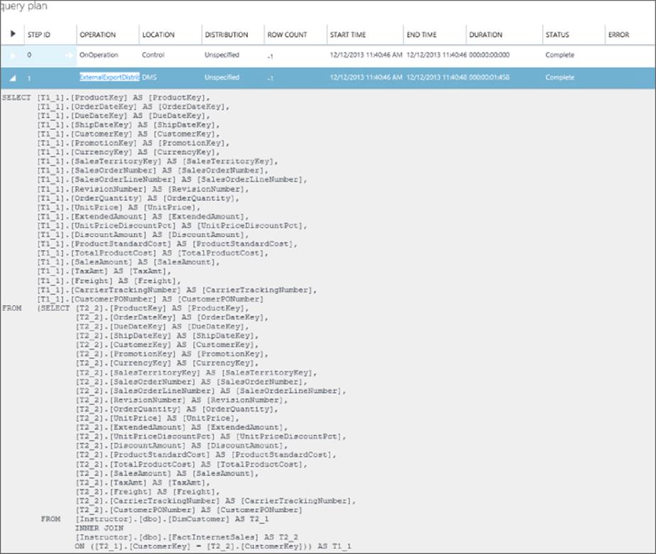
Figure 10.13 Exporting data using the DMS and its ExternalExportDistributedOperation

You can also see how the parallel export is achieved by looking at the files created in HDFS by PDW. You can see these files by querying the HDFS file system using the following command in the Hadoop console:

Hadoop fs -ls /files/HDFS_FactInternetSales

If you look at the Figure 10.14, you can clearly see that a naming convention has been applied to each file. This naming convention helps to explain the parallelism.

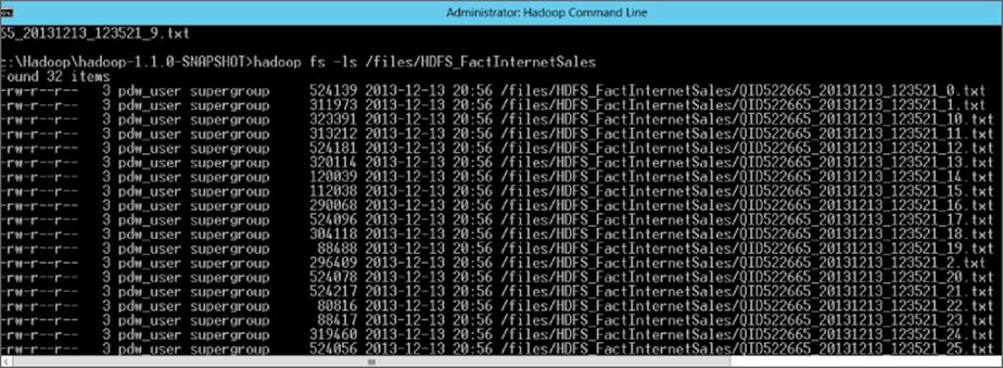
Figure 10.14 Viewing exported data from PDW in HDFS through the Hadoop Console

The naming convention of the file is as follows (see Table 10.5):

Table 10.5 HDFS File Naming Convention

QUERYID_DATE_TIME_DISTRIBUTION

We can conclude that PDW is creating one file per distribution and that this is how PDW is able to write the data out in parallel. Consequently, we can also conclude that if the data is skewed in PDW, the files in HDFS will be similarly skewed. By default, there will be three copies of the data, and the files will be constituted from 64MB blocks (because this is the block size). We can see the actual size and the number of replicas with our -ls command. The value 524139 shown in Figure 10.14 is the size in bytes for the first distribution (that is, distribution 0 or compute node 1 distribution A in PDW parlance). We can also see how many copies of this file we have from -ls command. Figure 10.14 shows the value 3 appearing on every row. It's located on the left after the file permissions and is followed by the name of the user (always pdw_user for data written by PDW) responsible for its creation. Sadly, the block size used isn't available through -ls.

What about replicated tables? Good question. Replicated tables export only to a single file, so in that sense there is no parallel export of a replicated table.

Aside from the ExternalExportDistributedOperation operation, it's basically the same suite of steps taken when an external table is created, including the collection of the table size and row count statistical information, courtesy of ExternalStatisticsOperation.

Remember that the external table persists after the CETAS operation. On the one hand, this is helpful for querying or importing the data later on. We also know that we have some statistical data associated with the table. On the other hand, it does prevent you from reexecuting this code (that is, you have to first drop the external table first). (I have to say that it would be really nice if you could just execute this code with a DROP_EXISTING instead, because remembering to drop the external table is a pain.)

There is one possible reason for not including DROP_EXISTING syntax in the CETAS statement. Simply dropping the external table does nothing to affect the data in Hadoop. This might lead to unexpected behavior for some people. If I did decide to drop the external table and simply reexecuted the CETAS query, I would in effect append the same data to the “table” in HDFS. Remember that the table in HDFS is merely a folder containing files of data. A simple export of data, via CETAS, pushes another new set of files to the same folder within HDFS, which effectively replicates the content. To first properly clean up the data and remove it from HDFS, I must execute a command in Hadoop like the one here:

Hadoop fs -rmr /files/HDFS_FactInternetSales

Now the data and the folder have been moved to the trash, as you can see in Figure 10.15 (IP address and port blacked out).

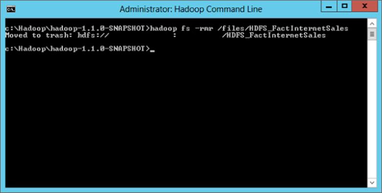
Figure 10.15 Cleaning up directories in Hadoop with -rmr

Perhaps a more complete extension to CETAS would be WITH (TRUNCATE, DROP_EXISTING). This would both remove the existing external table and fire the Hadoop file system -rmr operation to clean up the data residing in Hadoop before the next export. However, at this stage neither TRUNCATE nor DROP_EXISTING exist at this moment.

Business Use Cases for Polybase Today

One of the comments I've heard several times is that Microsoft tends to only talk about what is coming down the line. Although this is both interesting and brings much excitement, it often also leads to frustration as readers, listeners and viewers often end up feeling that there is no immediate use-case for the technology. I am going to try to address that in this section, at least in part. Therefore, in the following subsections, I discuss some of the ideas I've had for how to use Polybase, based purely on the building blocks we have today.

Archiving and Audit

The first scenario I want to suggest is an extension to the archiving solution Thomas Kejser proposed and that I highlighted earlier in this chapter. Thomas suggested that Hadoop and Hive could be a simple place to store source system data, which could both be easily queried and with Polybase now very easily rehydrated if needed. This would enable all sorts of warehouse replay functionality.

My proposed extension for this is to archive snapshot views of data. Suppose, for example, that a user queries a sensitive table. How do you track what the user saw at the time he saw it? One possible solution is to intercept the SELECT statement and instead prepend it with a CETAS statement, thus exporting the data into Hadoop creating a formal record of the data viewed.

This data could then be read from that file with a modified SELECT against the external table, thus guaranteeing that the same data is read as was recorded against the user accessing the data. These audit snapshots could be implemented in the database itself, but this can sometimes lead to a lot of data being generated and held in a relational store with little requirement to actually do anything with it. This is an attempted low-cost solution to that problem.

In summary, the advantages of this approach are as follows:

· Simple audit process

· Use of low-cost storage

· Reduced complexity for the database

· Removes storage capacity from the database

· Online retrieval if ever required

The primary disadvantage here is the network round-trip.

Data Subsetting and Obfuscation

Time for a variation on a theme: when you need to move data from one environment to another, it is often not a simple case of backup and restore. Consider moving data from production down to development or quality assurance environments. Often you don't want to move all the data, just a meaningful subset for representative testing volumes. More importantly, you want to ensure that no personally identifiable information is exposed in less-secure environments. Therefore, we need a way to both create obfuscated but meaningful subsets of production data.

One option is to leverage the export capabilities of Polybase to perform a high-performance data subsetting and obfuscation routine. Once exported, this data could then be picked up by other PDWs or even other systems from Hadoop. If required, one could also run additional algorithms over the data in Hadoop to provide further obfuscation to the data.

Data Hub/Broker

Like PDW, Hadoop can often be considered as a downstream system. In other words, it receives data from other data sources, which are then brought in for analysis.

Integrating that data into Hadoop does require some additional skills and possible tooling. However, you could mitigate that need by using PDW as a data hub and delivery mechanism for the warehouse and Hadoop environments. This would have some nice benefits:

· No new skills

· No new tools

· Consistency of data

· Streamlined operations through consolidated feeds

Speculating on the Future for Polybase

Sometimes it's worth doing some research and wider reading. You can occasionally come across some hidden gems that make a worthwhile pursuit an invaluable one. Bear this in mind as we dust off our crystal ball and “speculate” on the future for Polybase.

Partitioned Appliance

In the June 2013 sigmod whitepaper authored by Dr. David DeWitt and others titled “Split Query Processing in Polybase,” I unearthed the following information morsel: “ . . . there are tentative plans to allow customers to partition their appliances into disjoint Hadoop and PDW regions . . .”

This first comment largely speaks for itself. To me, it is clear that the PDW team plans to enable PDW customers to use scale units for Hadoop. I'd expect this to be in addition to the features we have seen in Polybase already. Consequently, as users, I think what we will have is a choice. We can either integrate with Hadoop that's configured inside the appliance and/or integrate with Hadoop outside of the appliance. That'd be a pretty impressive option don't you think? Other vendors tend to favor one deployment model and only work with a single distribution. As we look to the future, the agnostic architecture of Polybase is really starting to show its true worth.

However, before we delve a little deeper into this topic, there is another tidbit of information from the same whitepaper: “There are no plans currently to allow customers to co-locate a SQL Server instance and a Hadoop Datanode.”

This makes quite a bit of sense to me. The virtual machines used by PDW for the compute nodes are presized to consume almost all the resources available. Therefore, there isn't much compute processing room for the data nodes. Furthermore, you probably wouldn't want any unpredictable resource contention, which might be another reason to keep the two workloads “disjointed.”

One possible advantage of having Hadoop “inside” of PDW is that you might be able to have relational database management system (RDBMS)-like security over the data inside HDFS. As mentioned previously, security isn't exactly Hadoop's forte. However, I would imagine that I can only grant access privileges to people I want to be able to engage on the data, for example.

Another reason might be flexibility. Remember that PDW's configuration is almost completely virtual. The workload definition, for example, is in the compute nodes (a virtual machine). Would it be not be possible therefore to decide that I would like to have four compute PDW nodes with four data nodes one day and six compute and four data the next? Granted, the amount of data committed to any data node(s) would represent an obstacle (data would need to be rebalanced between the remaining compute nodes), but it would in theory at least be possible.

Earlier in the chapter we discussed having separate Hadoop environments for various user personas. A partitioned appliance could be a great location for our power user and consumer community grade data sets, giving them dedicated compute resources that would be very close to the enterprise data held in PDW. This workload isolation would also benefit the data scientists as they wouldn't need to worry about interference from corporate users as much. Naturally, Polybase would be the perfect fit for migrating the data between these Bronze, Silver, and Gold environments. Being able to leverage PDW's ultra-low latency Infiniband network would also come in extremely handy for those challenging ad-hoc queries.

Finally, manageability: from an operational perspective, will a single-managed appliance be more attractive than having two distributed systems and having to manage them separately? There's an opportunity for consolidated management and monitoring here for PDW and Hadoop using a single interface that goes beyond System Center Management Packs. The simplicity of an appliance experience will be a factor for some. That said, I am not sure about this one. Those who have more of a database-centric view of the world might be swayed by such an argument. Having a clean, consistent deployment of Hadoop without any configuration headaches as well having only “one throat to choke” when it comes to support may well prove attractive. However, it would very much depend on the PDW teams' execution focus and priorities. For this to prove really valuable to customers would be a lot of work I expect.

Architecture Versus Implementation

One positive aspect of the Polybase is that, architecturally, it makes no assumptions. Questions concerning data format, data location within HDFS, and number of data nodes, for example, are answered at runtime. This means that the Hadoop ecosystem and PDW can happily coexist without any dependencies.

However, not everything in that architectural vision made the cut when it came to the initial implementation that formed RTM of PDW 2012. One example concerns the format of the data in Hadoop. Although it is true to say that architecturally PDW makes no assumption on the format used to persist the data in HDFS (the HDFS Bridge provides the necessary abstraction), it is not true for the RTM Polybase implementation. At this moment, Polybase supports files in only delimited text format.

That said, I expect to see Polybase supporting other standard file formats and possibly even custom file formats in the future. As long as we can impose that structure on the underlying data file, we should be all good. One example that I could see in the near term is the optimized row columnar (ORC) file format, which has been the subject of much development through the stinger initiative and is very commonly used by Hive users.

Optimized Big Data Queries

In his keynote presentation “Polybase: What, Why, How” at the PASS Summit in 2012 (http://gsl.azurewebsites.net/Portals/0/Users/dewitt/talks/PolybasePass2012.pptx), Dr. DeWitt gave some indications to the roadmap of Polybase. At this illuminating session, he broke the roadmap into three phases. Phase 1 is what we have in PDW today, so I won't belabor that. Phase 2 was really focused on using the computational resources of the Hadoop cluster; selectively issuing MapReduce jobs to optimize queries instead of relying on the parallel import functionality that PDW has today. Phase 3 was much heavily caveated. Therefore, it's difficult to read too much into it. However, it was clear that a lot of thought is going into leveraging Hadoop 2.0, Yarn, and Tez. Could we see a more holistic optimizer? Perhaps we'll see PDW dynamically exporting data to Hadoop because it might be more efficient to process the data there for example. Who knows? Suddenly the crystal ball looks a little bit too blurry.

Let's step back to phase 2 then. While highlighting the opportunity for leveraging Hadoop's compute resources, Dr. DeWitt also highlighted several challenges that made me realize that this wasn't simply a case of just getting PDW to issue MapReduce jobs every time a Polybase query is received. In order to decide where and when to use MapReduce, PDW would need additional information fed into it so it could make an informed decision to use it or not. However, put simply, Hadoop did not hold the kind of data required by PDW. It was clearly not going to be a trivial task deriving this information either. We will discuss the kinds of data PDW shortly but first let's understand a bit more about how PDW optimizes a query.

Rather than use a rules engine, PDW uses a cost-based optimizer to determine how to resolve your query in the most efficient manner. Like SQL Server, we create statistics on key columns to help guide the optimizer. In PDW, we create stats on all columns involved in the following areas of a query:

· Joins

· Group by

· Where clause

· Order by

Having these statistical objects created on our tables helps PDW decide on the best MPP plan for your query. In some cases, especially for composite joins, we may even create multicolumn stats to help guide the optimizer further. A multicolumn statistic provides the density of the neighboring column(s) to the optimizer, which can help to influence the type of join chosen. Instead of a nested loop join, which is often undesirable and inefficient in a data warehouse, we might be able to influence the optimizer to choose a hash join, for example. All these techniques are great tuning options for data in your data warehouse.

Hadoop and HDFS do not even hold this basic information. Its approach to data analysis is more sledgehammer based. Remember the Hadoop mindset is to throw compute at the problem.

However, with a system such as Polybase, you really need the statistical information, and a whole lot more. Therefore, in addition to holding statistical information about data held in Hadoop, the Polybase engineers need access to additional information to determine the optimal plan. Consider this list for starters:

· Hadoop cluster size

· Network bandwidth to Hadoop cluster

· Utilization of resources on Hadoop

· Proximity of Hadoop cluster

· Selectivity of predicates for data held in Hadoop

· Semantic differences between Java and SQL

As Polybase evolves and both Hadoop and PDW mature, you could see some really interesting decisions being made. Is 90% of the data in Hadoop, for example? One answer could be to send the remaining data over to Hadoop and process the query there. Is Hadoop busy and data volume reasonable? Move the data to PDW. I am no query processor expert (far from it), but these kinds of possibilities are exciting!

Why Poly in Polybase?

If the sole objective of Polybase was to integrate with just HDFS, why call it Polybase? If we look at the definition of poly, which is “more than one; many or much” (according to the Collins Dictionary), is this not a clear signal of bigger things to come? Speaking personally for a moment, I'd love to be able to simply reference delimited files exposed on a Windows NTFS file system. I think that would be a really nice extension of this feature and would significantly strengthen PDW's data export functionality. However, I am sure that the cloud will factor into Polybase somewhere. Every product in the Microsoft Data Platform has to have a cloud strategy, and PDW is no exception. If on-premise Hadoop is the cold storage for PDW, could Azure be the deep freezer?

Thinking further ahead, who's is to say that Polybase couldn't be used to integrate with other systems such as SAP Hana or Oracle? After all, a cow has many stomachs. Why can't PDW have many engines? That's certainly something for you to chew on.

Summary

Well, that's about it for PDW and Polybase. I hope you found that interesting, and you learned a bit about PDW and why it is important to the world of data warehousing. However, more importantly, I hope that you are excited about the integration opportunities that Polybase offers us, both now and in the future. It's important to remember that only PDW offers Polybase and Hadoop integration.

Polybase is an enormously strategic piece of technology. Its holistic, agnostic architecture and approach to Hadoop integration opens up the relational world to a whole host of new opportunities. I hope you agree and will give much stronger consideration to PDW and its capabilities for your next project.

This is a rapidly changing and highly dynamic environment. I'm therefore expecting to see lots of great improvements and solutions in the months ahead. Remember PDW also updates with new features twice a year, so the next set of features are never far away!