MICROSOFT BIG DATA SOLUTIONS (2014)

Part IV. Working with Your Big Data

Chapter 9. Data Research and Advanced Data Cleansing with Pig and Hive

What You Will Learn in This Chapter

· Understanding the Difference Between Pig and Hive and When to Use Each

· Using Pig Latin Built-in Functions for Advanced Extraction, and Transforming and Loading Data

· Understanding the Various Types of Hive Functions Available

· Extending Hive with Map-reduce Scripts

· Creating Your Own Functions to Plug into Hive

All data processing on Hadoop essentially boils down to a map-reduce process. The mapping consists of retrieving the data and performing operations such as filtering and sorting. The reducing part of the process consists of performing a summary operation such as grouping and counting. Hadoop map-reduce jobs are written in programming languages such as Java and C#. Although this works well for developers with a programming background, it requires a steep learning curve for nonprogrammers. This is where Pig comes in to play. Another tool available to create and run map-reduce jobs in Hadoop is Hive. Like Pig, Hive relies on a batch-based, parallel-processing paradigm and is useful for querying, aggregating, and filtering large data sets.

This chapter covers both Pig and Hive and will help you to understand the strengths of each. You will also see how to extend Pig and Hive using functions and custom map-reduce scripts. In addition, the chapter includes hands-on activities to help you solidify the concepts presented.

Getting to Know Pig

Pig was originally developed as a research project within Yahoo! in 2006. It became popular with the user community as a way to increase productivity when writing map-reduce jobs. By 2007, Yahoo! decided to work with the open source community to develop Pig into a production-quality product. The open source community embraced the project, and additional features were added such as error handling, a streaming operator, parameter substitution, and binary comparators. Eventually, the entire codebase was rewritten to provide significant performance increases. With the growing popularity of Hadoop and Pig, the open source community continues to improve and augment Pig.

Today, Pig is a high-level scripting program used to create map-reduce functions that are translated to Java and run on a Hadoop cluster. The scripting language for Pig is called Pig Latin and is written to provide an easier way to write data-processing instructions. In the following sections, you'll learn more about Pig, including when to use Pig and how to use both built-in and user-defined functions.

The Difference Between Pig and Hive

The main difference between Pig and Hive is that Pig Latin, Pig's scripting language, is a procedural language, whereas HiveQL is a declarative language. This means that when using Pig Latin you have more control over how the data is processed through the pipeline, and the processing consists of a series of steps, in between which the data can be checked and stored. With HiveQL, you construct and run the statement as a whole, submitting it to a query engine to optimize and run the code. You have very little influence on the steps performed to achieve the result. Instead, you have faith that the query engine will choose the most efficient steps needed. If you have a programming background, you are probably more comfortable with and like the control you get using Pig Latin. However, if you a lot of experience with writing database queries, you will most likely feel more comfortable with HiveQL.

When to Use Pig

It is important that you use the right tool for the job. Although we have all used the side of a wrench to hammer in a nail, a hammer works much better! Pig is designed and tuned to process large data sets involving a number of steps. As such, it is primarily an extraction transform load (ETL) tool. In addition, like all Hadoop processing, it relies on map-reduce jobs that can be run in parallel on separate chunks of data and combined after the analysis to arrive at a result. For example, it would be ideal to look through massive amounts of data measurements like temperatures, group them by days, and reduce it to the max temperature by day. Another factor to keep in mind is the latency involved in the batch processing of the data. This means that Pig processing is suitable for post-processing of the data as opposed to real-time processing that occurs as the data is collected.

You can run Pig either interactively or in batch mode. Typically interactive mode is used during development. When you run Pig interactively, you can easily see the results of the scripts dumped out to the screen. This is a great way to build up and debug a multi-step ETL process. Once the script is built, you can save it to a text file and run it in batch mode using scheduling or part of a workflow. This generally occurs during production where scripts are run unattended during off-peak hours. The results can be dumped into a file that you can use for further analysis or as an input file for tools, such as PowerPivot, Power View, and Power Map. (You will see how these tools are used in Chapter 11, “Visualizing Big Data with Microsoft BI.”)

Taking Advantage of Built-in Functions

As you saw in Chapter 8, “Effective Big Data ETL with SSIS, Pig, and SQOOP,” Pig scripts are written in a script language called Pig Latin. Although it is a lot easier to write the ETL processing using Pig Latin than it is to write the low level map-reduce jobs, at some point the Pig Latin has to be converted into a map-reduce job that does the actual processing. This is where functions come into the picture. In Pig, functions process the data and are written in Java. Pig comes with a set of built-in functions to implement common processing tasks such as the following:

· Loading and storing data

· Evaluating and aggregating data

· Executing common math functions

· Implementing string functions

For example, the default load function PigStorage is used to load data into structured text files in UTF-8 format. The following code loads a file containing flight delay data into a relation (table) named FlightData:

FlightData = LOAD 'FlightPerformance.csv' using PigStorage(',');

Another built-in load function is JsonLoader. This is used to load JSON (JavaScript Object Notation)-formatted files. JSON is a text-based open standard designed for human-readable data interchange and is often used to transmit structured data over network connections. The following code loads a JSON-formatted file:

FlightData = LOAD ' FlightPerformance.json' using JsonLoader();

NOTE

For more information on JSON, see http://www.json.org/.

You can also store data using the storage functions. For example, the following code stores data into a tab-delimited text file (the default format):

STORE FlightData into 'FlightDataProcessed' using PigStorage();

Functions used to evaluate and aggregate data include IsEmpty, Size, Count, Sum, Avg, and Concat, to name a few. The following code filters out tuples that have an empty airport code:

FlightDataFiltered = Filter FlightData By IsEmpty(AirportCode);

Common math functions include ABS, CEIL, SIN, and TAN. The following code uses the CEIL function to round the delay times up to the nearest minute (integer):

FlightDataCeil = FOREACH FlightData

GENERATE CEIL(FlightDelay) AS FlightDelay2;

Some common string functions are Lower, Trim, Substring, and Replace. The following code trims leading and trailing spaces from the airport codes:

FlightDataTrimmed = FOREACH FlightData

GENERATE TRIM(AirportCode) AS AirportCode2;

Executing User-defined Functions

In the preceding section, you looked at some of the useful built-in functions available in Pig. Because these are built-in functions, you do not have to register the functions or use fully qualified naming to invoke them because Pig knows where the functions reside. It is recommended that you use the built-in functions if they meet your processing needs. However, these built-in functions are limited and will not always meet your requirements. In these cases, you can use user-defined functions (UDFs).

Creating your own functions is not trivial, so you should investigate whether a publicly available UDF could meet your needs before going to the trouble of creating your own. Two useful open source libraries containing prebuilt UDFs are PiggyBank and DataFu, discussed next.

PiggyBank

PiggyBank is a repository for UDFs provided by the open source community. Unlike with the built-in UDFs, you need to register the jar to use them. The jar file contains the compiled code for the function. Once registered, you can use them in your Pig scripts by providing the function's fully qualified name or use the define statement to provide an alias for the UDF. The following code uses the reverse function contained in the piggybank.jar file to reverse a string. The HCatLoader loads data from a table defined using HCatalog (covered in Chapter 7, “Expanding Your Capability with HBase and HCatalog”):

define reverse org.apache.pig.piggybank.evaluation.string.Reverse();

FlightData = LOAD 'FlightData'

USING org.apache.hcatalog.pig.HCatLoader();

FlightDataReversed = Foreach FlightData

Generate (origin, reverse(origin));

PiggyBank functions are organized into packages according to function type. For example, the org.apache.pig.piggybank.evaluation package contains functions for custom evaluation operations like aggregates and column transformations. The functions are further organized into subgroups by function. The org.apache.pig.piggybank.evaluation.string functions contain custom functions for string evaluations such as the reverse seen earlier. In addition to the evaluation functions, there are functions for comparison, filtering, grouping, and loading/storing.

DataFu

DataFu was developed by LinkedIn to aid them in analyzing their big data sets. This is a well-tested set of UDFs containing functions for data mining and advanced statistics. You can download the jar file from www.wiley.com/go/microsoftbigdatasolutions. To use the UDFs, you complete the same process as you do with the PiggyBank library. Register the jar file so that Pig can locate it and define an alias to use in your script. The following code finds the median of a set of measures:

DEFINE Median datafu.pig.stats.Median();

TempData = LOAD '/user/test/temperature.txt'

using PigStorage() AS (dtstamp:chararray, sensorid:int, temp:double);

TempDataGrouped = Group TempData ALL;

MedTemp = ForEach TempDataGrouped

{ TempSorted = ORDER TempData BY temp;

GENERATE Median(TempData.temp);};

Using UDFs

You can set up Hortonworks Data Platform (HDP) for Windows on a development server to provide a local test environment that supports a single-node deployment. (For a detailed discussion of installing the Hadoop development environment on Windows, see Chapter 3, “Installing HDInsight.”)

NOTE

To complete the following activity, you need to download and install the HDP for Windows from Hortonworks or the HDInsight Emulator from Microsoft.

After you have installed the environment, you should see three icons on the desktop for interacting with the Hadoop service. The NameNode maintains the directory files in the Hadoop Distributed File System (HDFS). It also keeps track of where the data files are kept in a Hadoop cluster. Figure 9.1 shows the information displayed when you click the NameNode icon.

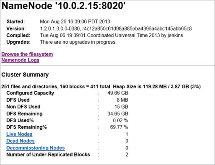
Figure 9.1 Displaying the NameNode information

Additional links appear on the NameNode information page for browsing the file system and log files and for additional node information. Figure 9.2 shows the files in the /user/Dan directory.

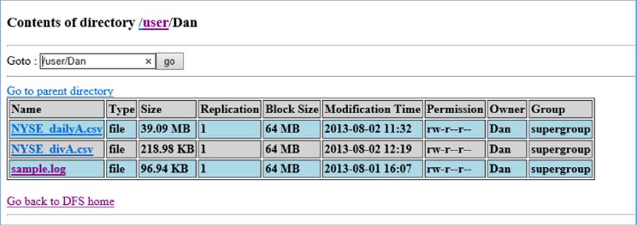
Figure 9.2 Exploring the directory file listing

You can also drill in to see the contents of a data file, as shown in Figure 9.3.

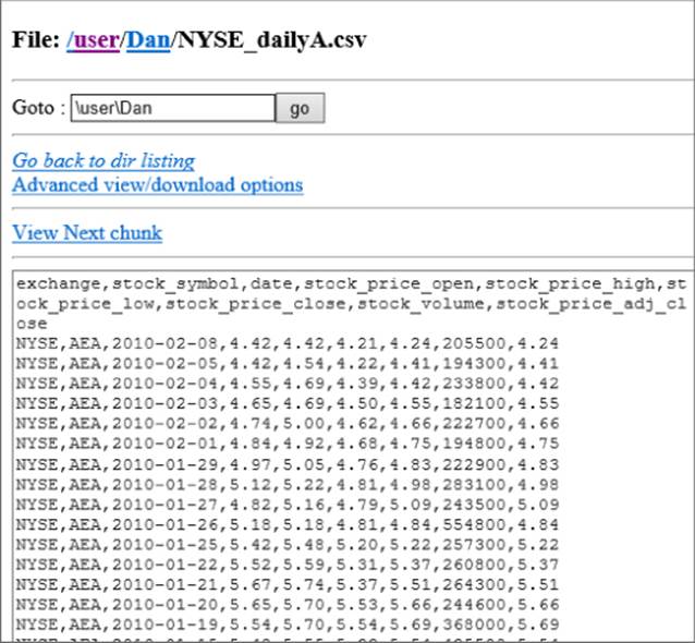
Figure 9.3 Drilling into a data file

The Hadoop Map-Reduce Status icon launches the Map/Reduce Administration page. This page provides useful information about the map-reduce jobs currently running, scheduled to run, or having run in the past. Figure 9.4 shows summary information for a job that was run on the cluster.

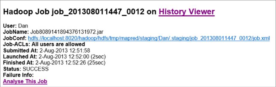
Figure 9.4 Viewing job summary stats

The third link is a shortcut to the Hadoop command-line console window displaying the Hadoop command prompt. Using this console, you can build and issue map-reduce jobs and issue Hadoop File System (FS) commands. You can also use this console to administer the Hadoop cluster. Figure 9.5 shows the Hadoop console being used to list the files in a directory.

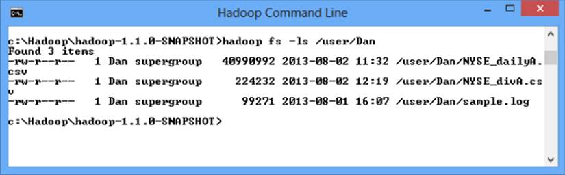
Figure 9.5 Using the Hadoop command-line console

After installing and setting up the environment, you are now ready to implement an ETL process using Pig. In addition you will use UDFs exposed by PiggyBank and DataFu for advanced processing.

The four basic steps contained in this activity are:

1. Loading the data.

2. Running Pig interactively with Grunt.

3. Using PiggyBank to extract time periods.

4. Using DataFu to implement some advanced statistical analysis.

Loading Data

The first thing you need to do is load a data file. You can download a sample highway traffic data file at www.wiley.com/go/microsoftbigdatasolutions. Once the data file is downloaded, you can load it into HDFS using the Hadoop command-line console. Open the console and create a directory for the file using the following code:

hadoop fs –mkdir /user/test

Next, use the following command to load the traffic.txt file into the directory:

Hadoop fs –copyFromLocal C:\SampleData\traffic.txt /user/test

Once the file is copied into the Hadoop directory, you should be able to browse to the directory and view the data using the Hadoop NameNode link. Figure 9.6 shows the file open in the NameNode browser.

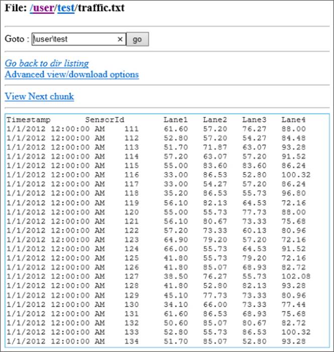
Figure 9.6 Viewing the traffic.txt data

Running Pig Interactively with Grunt

From the bin folder of the Pig install folder (hdp\hadoop\pig\bin), open the Pig command-line console to launch the Grunt shell. The Grunt shell enables you to run Pig Latin interactively and view the results of each step. Enter the following script to load and create a schema for the traffic data:

SpeedData = LOAD '/user/test/traffic.txt'

using PigStorage() AS (dtstamp:chararray, sensorid:int, speed:double);

Dump the results to the screen:

DUMP SpeedData;

By doing so, you can run a map-reduce job that outputs the data to the console window. You should see data similar to Figure 9.7, which shows the tuples that make the set of data.

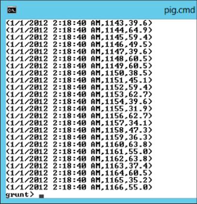
Figure 9.7 Dumping results to the console window

Using PiggyBank to Extract Time Periods

The next step in analyzing the data is to group it into different date/time buckets. To accomplish this, you use functions defined in the piggybank.jar file. If that file is not already installed, you can either download and compile the source code or download a compiled jar file from www.wiley.com/go/microsoftbigdatasolutions. Along with the piggybank.jar file, you need to get a copy of the joda-time-2.2.jar file from www.wiley.com/go/microsoftbigdatasolutions, which is referenced by the piggybank.jar file.

Place the jar files in a directory accessible to the Pig command-line console; for example, you can place it in the same directory as the pig.jar file. Now you can register and alias the PiggyBank functions in your Pig Latin scripts. The first function you use here is theCustomFormatToISO. This function converts the date/time strings in the file to a standard ISO format:

DEFINE Convert

org.apache.pig.piggybank.evaluation.datetime.convert.CustomFormatToISO;

Use the following code to load and convert the date/time values:

SpeedData = LOAD '/user/test/traffic.txt' using PigStorage()

AS (dtstamp:chararray, sensorid:int, speed:double);

SpeedDataFormat = FOREACH SpeedData Generate dtstamp,

Convert(dtstamp,'MM/dd/YYYY hh:mm:ss a') as dtISO;

Dump SpeedDataFormat;

After the job completes, you should see data similar to the data shown in Figure 9.8.

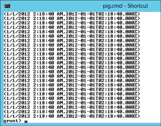
Figure 9.8 Reformatted date/times

Now that you have the dates in ISO format, you can easily strip out the day and hour from the date. Use the following code to create the day and hour fields. The output should match Figure 9.9:

DEFINE Convert

org.apache.pig.piggybank.evaluation.datetime.convert.CustomFormatToISO;

DEFINE SubString org.apache.pig.piggybank.evaluation.string.SUBSTRING;

SpeedData = LOAD '/user/test/trafic.txt' using PigStorage()

AS (dtstamp:chararray, sensorid:int, speed:double);

SpeedDataFormat = FOREACH SpeedData Generate dtstamp,

Convert(dtstamp,'MM/dd/YYYY hh:mm:ss a') as dtISO, speed;

SpeedDataHour = FOREACH SpeedDataFormat

Generate dtstamp, SubString(dtISO,5,7) as day,

SubString(dtISO,11,13) as hr, speed;

Dump SpeedDataHour;

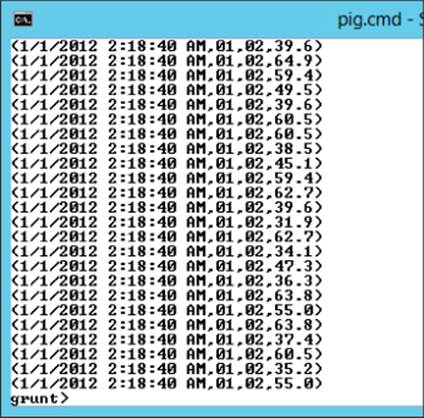
Figure 9.9 Splitting day and hour from an ISO date field

Now you can group the data by hour and get the maximum, minimum, and average speed recorded during each hour (see Figure 9.10):

SpeedDataGrouped = Group SpeedDataHour BY hr;

SpeedDataAgr = FOREACH SpeedDataGrouped

GENERATE group, MAX(SpeedDataHour.speed),

MIN(SpeedDataHour.speed), AVG(SpeedDataHour.speed);

Dump SpeedDataAgr;

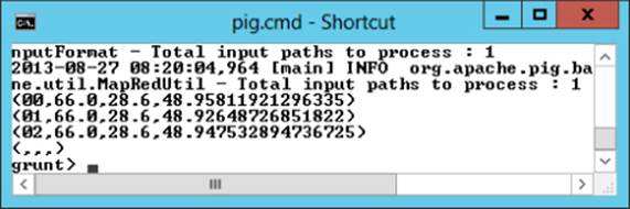
Figure 9.10 Speed data aggregated by hour

Using DataFu for Advanced Statistics

Even though Pig contains some rudimentary statistical UDFs you can use to analyze the data, you often need to implement advanced statistical techniques to accurately process the data. For example, you might want to eliminate outliers in your data. To determine the outliers, you can use the DataFu Quantile function and compute the 10th and 90th percentile values.

To use the DataFu UDFs, download the datafu.jar file from www.wiley.com/go/microsoftbigdatasolutions and place it in the same directory as the piggybank.jar file. You can now reference the jar file in your script. Define an alias for the Quantile function and provide the quantile values you want to calculate:

DEFINE Quantile datafu.pig.stats.Quantile('.10','.90');

Load and group the data:

SpeedData = LOAD '/user/test/traffic.txt' using PigStorage()

AS (dtstamp:chararray, sensorid:int, speed:double);

SpeedDataGrouped = Group SpeedData ALL;

Pass sorted data to the Quantile function and dump the results out to the command-line console (see Figure 9.11). Using this data, you can then write a script to filter out the outliers:

QuantSpeeds = ForEach SpeedDataGrouped

{ SpeedSorted = ORDER SpeedData BY speed;

GENERATE Quantile(SpeedData.speed);};

Dump QuantSpeeds;

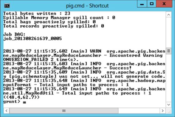
Figure 9.11 Finding the 10th and 90th percentile

Now that you know how to use UDFs to extend the functionality of Pig, it is time to take it a step further and create your own UDF.

Building Your Own UDFs for Pig

Unless you are an experienced Java programmer, writing your own UDF is not trivial, as mentioned earlier. However, if you have experience in another object-oriented programming language such as C#, you should be able to transition to writing UDFs in Java without too much difficulty. One thing you may want to do to make things easier is to download and install a Java interface development environment (IDE) such as Eclipse (http://www.eclipse.org/). If you are used to working in Visual Studio, you should be comfortable developing in Eclipse.

You can create several types of UDFs, depending on the functionality. The most common type is the eval function. An eval function accepts a tuple as an input, completes some processing on it, and sends it back out. They are typically used in conjunction with aFOREACH statement in HiveQL. For example, the following script calls a custom UDF to convert string values to lowercase:

Define lcase com.BigData.hadoop.pig.SampleUDF.Lower;

FlightData = LOAD '/user/test/FlightPerformance.csv'

using PigStorage(',')

as (flight_date:chararray,airline_cd:int,airport_cd:chararray,

delay:int,dep_time:int);

Lower = FOREACH FlightData GENERATE lcase(airport_cd);

To create the UDF, you first add a reference to the pig.jar file. After doing so, you need to create a class that extends the EvalFunc class. The EvalFunc is the base class for all eval functions. The import statements at the top of the file indicate the various classes you are going to use from the referenced jar files:

import java.io.IOException;

import org.apache.pig.EvalFunc;

import org.apache.pig.data.Tuple;

public class Lower extends EvalFunc<String>

{

}

The next step is to add an exec function that implements the processing. It has an input parameter of a tuple and an output of a string:

public String exec(Tuple arg0) throws IOException

{

if (arg0 == null || arg0.size() == 0)

return null;

try

{

String str = (String)arg0.get(0);

return str.toLowerCase();

}

catch(Exception e)

{

throw new

IOException("Caught exception processing input row ", e);

}

The first part of the code checks the input tuple to make sure that it is valid and then uses a try-catch block. The try block converts the string to lowercase and returns it back to the caller. If an error occurs in the try block, the catch block returns an error message to the caller.

Next, you need to build the class and export it to a jar file. Place the jar file in the Pig directory, and you are ready to use it in your scripts.

Another common type of function is the filter function. Filter functions are eval functions that return a Boolean result. For example, the IsPositive function is used here to filter out negative and zero-delay values (integers):

Define isPos com.BigData.hadoop.pig.SampleUDF.isPositive;

FlightData = LOAD '/user/test/FlightPerformance.csv'

using PigStorage(',')

as (flight_date:chararray,airline_cd:int,airport_cd:chararray,

delay:int,dep_time:int);

PosDelay = Filter FlightData BY isPos(delay);

The code for the isPositive UDF is shown here:

package com.BigData.hadoop.pig.SampleUDF;

import java.io.IOException;

import org.apache.pig.FilterFunc;

import org.apache.pig.data.Tuple;

public class isPositive extends FilterFunc {

@Override

public Boolean exec(Tuple arg0) throws IOException {

if (arg0 == null || arg0.size() != 1)

return null;

try

{

if (arg0.get(0) instanceof Integer)

{

if ((Integer)arg0.get(0)>0)

return true;

else

return false;

}

else

return false;

}

catch(Exception e)

{

throw new IOException

("Caught exception processing input row ", e);

}

It extends the FilterFunc class and includes an exec function that checks to confirm whether the tuple passed in is not null and makes sure that it has only one member. It then confirms whether it is an integer and returns true if it is greater than zero; otherwise, it returns false.

Some other UDF types are the aggregation, load, and store functions. The functions shown here are the bare-bones implementations. You also need to consider error handling, progress reporting, and output schema typing. For more information on custom UDF creation, consult the UDF manual on the Apache Pig wiki (http://wiki.apache.org/pig/UDFManual).

Using Hive

Another tool available to create and run map-reduce jobs in Hadoop is Hive. One of the major advantages of Hive is that it creates a relational database layer over the data files. Using this paradigm, you can work with the data using traditional querying techniques, which is very beneficial if you have a SQL background. In addition, you do not have to worry about how the query is translated into the map-reduce job. There is a query engine that works out the details of what is the most efficient way of loading and aggregating the data.

In the following sections you will gain an understanding of how to perform advanced data analysis with Hive. First you will look at the different types of built-in Hive functions available. Next, you will see how to extend Hive with custom map-reduce scripts written in Python. Then you will go one step further and create a UDF to extend the functionality of Hive.

Data Analysis with Hive

One strong point of HiveQL is that it contains a lot of built-in functions that assist you in your data analysis. There are a number of mathematical, collection, type conversion, date, and string functions. Most of the functions that are in the SQL language have been included in HiveQL. For example, the following HiveQL counts the flights and finds the maximum delay at each airport from the flightdata table. Figure 9.12 shows the output in the Hive console:

Select airport_cd, count(*), max(delay)

from flightdata group by airport_cd;

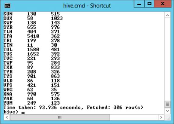
Figure 9.12 Flight counts and maximum delays

Types of Hive Functions

Hive has several flavors of functions you can work with, including the following:

· UDFs

· UDAFs (user-defined aggregate functions)

· UDTFs (user-defined table-generating functions)

UDFs work on single rows at a time and consist of functions such as type conversion, math functions, string manipulation, and date/time functions. For example, the following Hive query uses the date function to get the day from the flightdate field:

Select day(flightdate), airport_cd, delay

from flightdata where delay > 100;

Whereas UDFs work on single rows at a time and processing occurs on the map side of the processing, UDAFs work on buckets of data and are implemented on the reduce side of the processing. For example, you can use the built-in UDAF count and max to get the delay counts and maximum delays by day:

Select day(flightdate), count(*), max(delay)

from flightdata group by day(flightdate);

Another type of function used in Hive is a UDFT. This type of function takes a single-row input and produces multiple-row outputs. These functions are useful for taking a column containing an array that needs to be split out into multiple rows. Hive's built-in UDFTs include the following:

· The explode function, which takes an array as input and splits it out into multiple rows.

· The json_tuple function, which is useful for querying JSON-formatted nodes. It takes the JSON node and splits out the child nodes into separate rows into a virtual table for better processing performance.

· The parse_url_tuple function, which takes a URL and extracts parts of a URL string into multiple rows in a table structure.

The file shown in Figure 9.13 contains student data in JSON format.

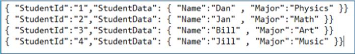
Figure 9.13 JSON formatted data

To parse the values from the JSON nodes, you use the json_tuple function in combination with the lateral view operator to create a table:

Select b.studentid, b.studentdata from studentdata a lateral view

json_tuple(a.jstring,'StudentId','StudentData') b

as studentid, studentdata;

Figure 9.14 shows the query output.

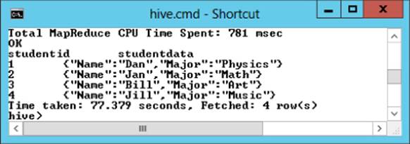
Figure 9.14 Parsing JSON data

Notice that this query did not parse out the nested JSON data from each row. To query the nested data, you need to add an additional lateral view:

Select b.studentid, c.name, c.major from studentdata a lateral view

json_tuple(a.jstring,'StudentId','StudentData') b

as studentid, studentdata

lateral view json_tuple(b.studentdata,'Name','Major') c as name, major;

Figure 9.15 shows the output with the nested JSON data parsed out into separate columns.

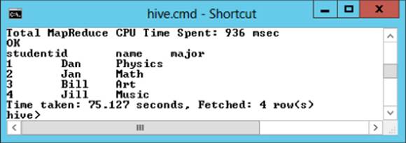
Figure 9.15 Parsing out nested data

Now that you have expanded out the nested data, you can analyze the data using reduce functions such as counting the number of students in each major.

Extending Hive with Map-reduce Scripts

There are times when you need to create a custom data-processing transformation that is not easy to achieve using HiveQL but fairly easy to do with a scripting language. This is particularly useful when manipulating if the result of the transform produces a different number of columns or rows than the input. For example, you want to split up an input column into several output columns using string-parsing functions. Another example is a column containing a set of key/value pairs that need to be split out into their own rows.

The input values sent to the script will consist of tab-delimited strings, and the output values should also come back as tab-delimited strings. Any null values sent to the script will be converted to the literal string \N to differentiate it from an empty string.

Although technically you can create your script in any scripting language, Pearl and Python seem to be the most popular. The code shown in Figure 9.16 is an example Python script that takes in a column formatted as hh:mm:ss and splits it into separate columns for hour, minute, and second.

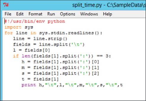
Figure 9.16 Python script for splitting time

To call this script from HiveQL, you use the TRANSFORM clause. You need to provide the TRANSFORM clause, the input data, output columns, and map-reduce script file. The following code uses the previous script. It takes an input of a time column and a log level and parses the time. Figure 9.17 shows the output:

add file c:\sampledata\split_time.py;

SELECT TRANSFORM(l.t4, l.t2) USING 'python split_time.py'

AS (hr,loglevel,min,sec,fulltime) from logs l;

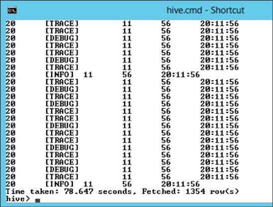
Figure 9.17 Splitting the time into hours, minutes, and seconds

The preceding script was a mapping script. You can also create reduce scripts for your custom processing. A reduce script takes tab-delimited columns from the input and produces tab-delimited output columns just like a map script. The difference is the reduce script combines rows in the process, and the rows out should be less than the rows put in. To run a reduce script, you need to have a mapping script. The mapping script provides the key/value pairs for the reducer. The Python script in Figure 9.18 is a mapping script that takes the input and checks whether it starts with a [ character. If it does, it outputs it to a line and gives it a count of one.

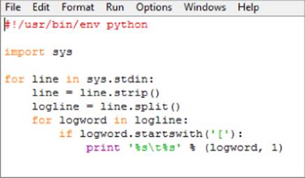
Figure 9.18 Mapping logging levels

Figure 9.19 shows a sample output from the script.

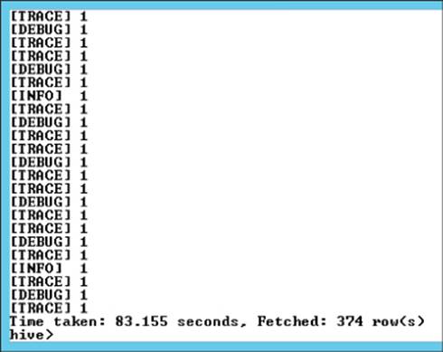
Figure 9.19 Mapping output

The output from the map script is fed into the reduce script, which counts the occurrence of each log level and returns the total count for each log level on a new line. Figure 9.20 shows the code for the reduce script.

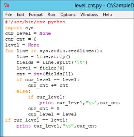
Figure 9.20 Reduce script to aggregate log level counts

You combine the map and reduce script into your HiveQL where the output from the mapper is the input for the reducer. The cluster by statement is used to partition and sort the output of the mapping by the loglevel key. The following code processes the log files through the custom map and reduce scripts:

add file c:\sampledata\map_loglevel.py;

add file c:\sampledata\level_cnt.py;

from (from log_table SELECT TRANSFORM(log_entry)

USING 'python map_loglevel.py'

AS (loglevel,cnt) cluster by loglevel) map_out

Select Transform(map_out.loglevel,map_out.cnt)

using 'python level_cnt.py' as level, cnt;

Another way to call the scripts is by using the map and reduce statements, which are an alias for the TRANSFORM statement. The following code calls the scripts using the map and reduce statements and loads the results into a script_test table:

add file c:\sampledata\map_loglevel.py;

add file c:\sampledata\level_cnt.py;

from (from log_table Map log_entry USING 'python map_loglevel.py'

AS loglevel, cnt cluster by loglevel) map_out

Insert overwrite table script_test Reduce map_out.loglevel, map_out.cnt

using 'python level_cnt.py' as level, cnt;

Figure 9.21 shows the aggregated counts of the different log levels.

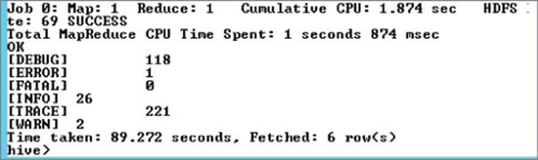
Figure 9.21 Output from the map-reduce scripts

Creating a Custom Map-reduce Script

In this exercise, we create a custom mapping script that takes a set of four measurements and returns the maximum value of the four. Figure 9.22 shows the input file, which you can download from www.wiley.com/go/microsoftbigdatasolutions.

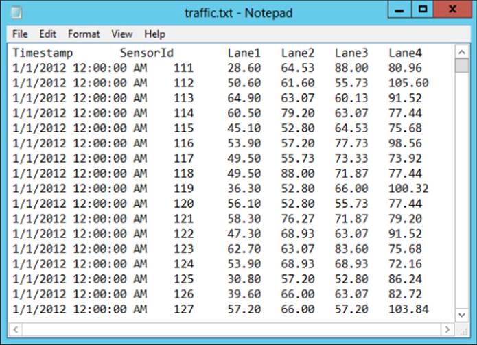
Figure 9.22 Input traffic data

Open your favorite text editor and enter the following code. Make sure to pay attention to the indenting:

#!/usr/bin/env python

import sys

for line in sys.stdin.readlines():

line = line.strip()

fields = line.split('\t')

time = fields[0]

sensor= fields[1]

maxvalue = max(fields[2:5])

print time,"\t",sensor,"\t",maxvalue

Save the file as get_maxValue.py in a reachable folder (for example, C:\SampleData). In the Hive command-line console, create a speeds table and load the data from traffic.txt into it:

CREATE TABLE speeds(recdate string, sensor string, v1 double, v2 double,

v3 double, v4 double) ROW FORMAT DELIMITED FIELDS TERMINATED BY '\t';

LOAD DATA LOCAL INPATH 'c:\sampledata\traffic.txt'

OVERWRITE INTO TABLE speeds;

Add a reference to the file and the TRANSFORM statement to call the script:

add file C:\SampleData\get_maxValue.py;

SELECT TRANSFORM(s.recdate,s.sensor,s.v1,s.v2,s.v3,s.v4)

USING 'python get_maxValue.py'

AS (recdate,sensor,maxvalue) FROM speeds s;

The data output should look similar to Figure 9.23.

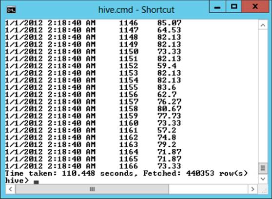
Figure 9.23 Output of the get_maxValue.py script

Creating Your Own UDFs for Hive

As mentioned previously, Hive contains a number of function types depending on the processing involved. The simplest type is the UDF, which takes a row in, processes it, and returns the row back. The UDAF is a little more involved because it performs an aggregation on input values and reduces the number of rows coming out. The other type of function you can create is the UDTF, which takes a row in and parses it out into a table.

If you followed along in the earlier section on building custom UDFs for Pig, you will find that building UDFs for Hive is a similar experience. First, you create a project in your favorite Java development environment. Then, you add a reference to the hive-exec.jarand the hive-serde.jar files. These are located in the hive folder in the lib subfolder. After you add these references, you add an import statement to the org.apache.hadoop.hive.ql.exec.UDF class and extend it with a custom class:

package Com.BigData.hadoop.hive.SampleUDF;

import org.apache.hadoop.hive.ql.exec.UDF;

public class OrderNums extends UDF{

}

The next step is to add an evaluate function that will do the processing and return the results. The following code processes the two integers passed in and returns the larger value. If they are equal it returns null. Because you are using the IntWritable class, you need to add an import for pointing to the org,apache.hadoop.io.IntWritable class in the Hadoop-core.jar file:

package Com.BigData.hadoop.hive.SampleUDF;

import org.apache.hadoop.io.IntWritable;

import org.apache.hadoop.hive.ql.exec.UDF;

public class GetMaxInt extends UDF{

public IntWritable evaluate(IntWritable x, IntWritable y)

{

if (x.get()>y.get())

return x;

else if (x.get()<y.get())

return y;

else

return null;

}

After creating and compiling the code into a jar file, deploy it to the hive directory. Once deployed you add the file to the hive class path and create an alias for the function using the Hive command line:

add jar C:\hdp\hadoop\hive-0.11.0.1.3.0.0-0380\lib\SampleUDF.jar;

create temporary function GetMaxInt as

'Com.BigData.hadoop.hive.SampleUDF.GetMaxInt';

You can now call the UDF in your HiveQL. Pass in two integers to get the larger value:

select f1, f2, GetMaxInt(f1,f2) from TestData;

Figure 9.24 shows the resulting output.

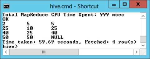
Figure 9.24 Sample UDF output

Once you are comfortable creating custom UDFs for Hive, you can investigate creating UDAFs and UDTFs. You can find more information about creating custom functions on the Apache Hive Wiki (https://cwiki.apache.org/confluence/display/Hive/Home).

Summary

In this chapter, you saw how Pig and Hive are used to apply data processing on top of Hadoop. You can use these tools to perform complex extracting, transformation, and loading (ETL) of your big data. Both of these tools process the data using functions created in Java code. Some of these functions are part of the native functionality of the toolset and are ready to use right out of the box. Some of the functions you can find through the open source community. You can download and install the jar files for these libraries and use them to extend the native functionality of your scripts. If you are comfortable programming in Java, you can even create your own functions to extend the functionality to meet your own unique processing requirements.

One takeaway from this chapter should be an appreciation of how extendable Pig Latin and HiveQL are at using pluggable interfaces. This chapter might even jump-start you to investigate further the process of creating and maybe even sharing your own custom function libraries.