Excel® 2016 Formulas and Functions (2016)
Part III: Building Business Models
14. Analyzing Data with PivotTables
In This Chapter
What Are PivotTables?
Building PivotTables
Working with PivotTable Subtotals
Changing the Data Field Summary Calculation
Creating Custom PivotTable Calculations
Using PivotTable Results in a Worksheet Formula
Tables and external databases can contain hundreds or even thousands of records. Analyzing that much data can be a nightmare without the right kinds of tools. To help you, Excel offers a powerful data analysis tool called a PivotTable. This tool enables you to summarize hundreds of records in a concise tabular format. You can then manipulate the layout of the table to see different views of your data. This chapter introduces you to PivotTables and shows you various ways to use them with your own data. Because this is a book about Excel formulas and functions, I don’t go into tons of detail on building and customizing PivotTables. Instead, I focus on the extensive work you can do with built-in and custom PivotTable calculations.
What Are PivotTables?
To understand PivotTables, you need to see how they fit in with Excel’s other database analysis features. Database analysis has several levels of complexity. The simplest level involves the basic lookup and retrieval of information. For example, if you have a database that lists the company sales reps and their territory sales, you could search for a specific rep to look up the sales in that rep’s territory.
The next level of complexity involves more sophisticated lookup and retrieval systems, in which the criteria and extraction techniques discussed in Chapter 13, “Analyzing Data with Tables,” are used. You can then apply subtotals and the table functions (also described in Chapter 13) to find answers to your questions. For example, suppose that each sales territory is part of a larger region, and you want to know the total sales in the East region. You could either subtotal by region or set up your criteria to match all territories in the East region and use the DSUM() function to get the total. To get more specific information, such as total East region sales in the second quarter, you just add the appropriate conditions to your criteria.
The next level of database analysis involves applying a single question to multiple variables. For example, if the company in the preceding example has four regions, you might want to see separate totals for each region, broken down by quarter. One solution would be to set up four different criteria and four different DSUM() functions. But what if there were a dozen regions? Or a hundred? Ideally, you need some way of summarizing the database information into a sales table that has a row for each region and a column for each quarter. This is exactly what PivotTables do and, as you’ll see in this chapter, you can create your own PivotTables with just a few mouse clicks.
How PivotTables Work
In the simplest case, PivotTables work by summarizing the data in one field (called a data field) and breaking it down according to the data in another field. The unique values in the second field (called the row field) become the row headings. For example, Figure 14.1 shows a table of sales by sales representatives. With a PivotTable, you can summarize the numbers in the Sales field (the data field) and break them down by Region (the row field). Figure 14.2 shows the resulting PivotTable. Notice how Excel uses the four unique items in the Region field (East, Midwest, South, and West) as row headings.
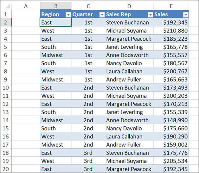
Figure 14.1 A table of sales by sales representatives.
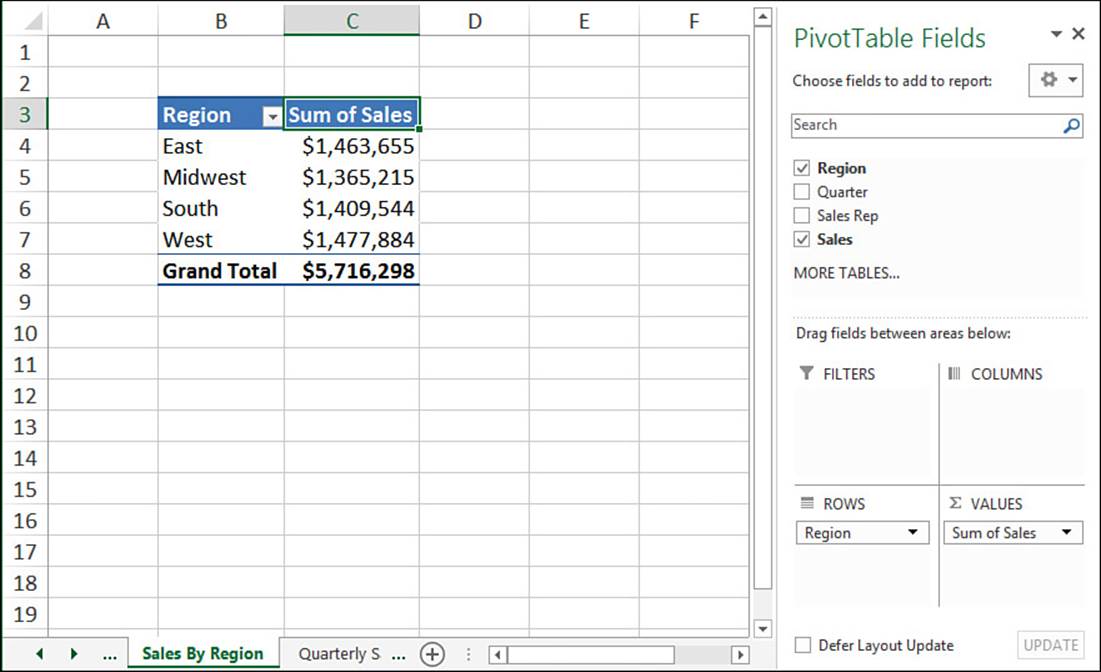
Figure 14.2 A PivotTable showing total sales by region.
Note
You can download this chapter’s sample workbooks at www.mcfedries.com/books/book.php?title=excel-2016-formulas-and-functions.
You can further break down your data by specifying a third field (called the column field) to use for column headings. Figure 14.3 shows the resulting PivotTable with the four unique items in the Quarter field (1st, 2nd, 3rd, and 4th) used to create the columns.
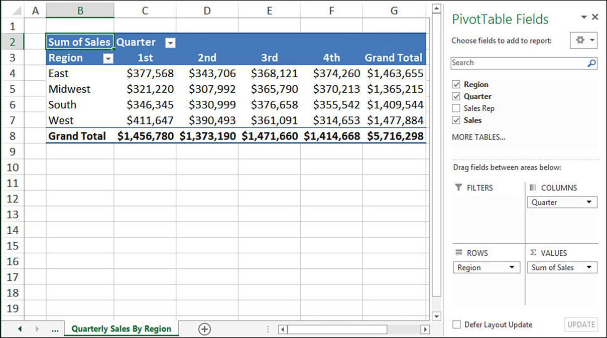
Figure 14.3 A PivotTable showing sales by region for each quarter.
The big news with PivotTables is the pivoting feature. You can use it to see different views of your data. For example, you can drag the column field over to the row field area, as shown in Figure 14.4. As you can see, the result is that the table shows each region as the main row category, with the quarters as regional subcategories.
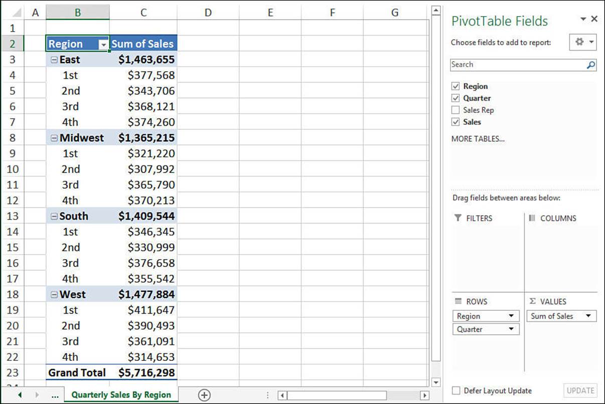
Figure 14.4 You can drag row or column fields to pivot the data and get a different view.
Some PivotTable Terms
PivotTables have their own terminology, so here’s a quick glossary of some terms you need to become familiar with:
![]() Data source—The original data. You can use a range, a table, imported data, or an external data source.
Data source—The original data. You can use a range, a table, imported data, or an external data source.
![]() Field—A category of data, such as Region, Quarter, or Sales. Because most PivotTables are derived from tables or databases, a PivotTable field is directly analogous to a table or database field.
Field—A category of data, such as Region, Quarter, or Sales. Because most PivotTables are derived from tables or databases, a PivotTable field is directly analogous to a table or database field.
![]() Label—An element in a field.
Label—An element in a field.
![]() Row field—A field with a limited set of distinct text, numeric, or date values to use as row labels in the PivotTable. In the preceding example, Region is the row field.
Row field—A field with a limited set of distinct text, numeric, or date values to use as row labels in the PivotTable. In the preceding example, Region is the row field.
![]() Column field—A field with a limited set of distinct text, numeric, or date values to use as column labels for the PivotTable. In the PivotTable shown in Figure 14.3, the Quarter field is the column field.
Column field—A field with a limited set of distinct text, numeric, or date values to use as column labels for the PivotTable. In the PivotTable shown in Figure 14.3, the Quarter field is the column field.
![]() Filter—A field with a limited set of distinct text, numeric, or date values that you use to filter the PivotTable view. For example, you could use the Sales Rep field as the filter. Selecting a different sales rep filters the table to show data only for that person.
Filter—A field with a limited set of distinct text, numeric, or date values that you use to filter the PivotTable view. For example, you could use the Sales Rep field as the filter. Selecting a different sales rep filters the table to show data only for that person.
![]() PivotTable items—The items from the source list used as row, column, and page labels.
PivotTable items—The items from the source list used as row, column, and page labels.
![]() Data field—A field that contains the data you want to summarize in the table.
Data field—A field that contains the data you want to summarize in the table.
![]() Data area—The interior section of the table, in which the data summaries appear.
Data area—The interior section of the table, in which the data summaries appear.
![]() Layout—The overall arrangement of fields and items in the PivotTable.
Layout—The overall arrangement of fields and items in the PivotTable.
Building PivotTables
PivotTables look complex to build, but creating a basic PivotTable takes just a few steps. You can also build fancier PivotTables; Excel offers a wide range of options, styles, and features on the Ribbon.
Building a PivotTable from a Table or Range
The most common source for a PivotTable is an Excel table, although you can also use data that’s set up as a regular range. You can use just about any table or range to build a PivotTable, but the best candidates for PivotTables exhibit two main characteristics:
![]() At least one of the fields contains groupable data. That is, the field contains data with a limited number of distinct text, numeric, or date values. In the Sales worksheet shown in Figure 14.1, the Region field is perfect for a PivotTable because, despite having dozens of items, it has only four distinct values: East, West, Midwest, and South.
At least one of the fields contains groupable data. That is, the field contains data with a limited number of distinct text, numeric, or date values. In the Sales worksheet shown in Figure 14.1, the Region field is perfect for a PivotTable because, despite having dozens of items, it has only four distinct values: East, West, Midwest, and South.
![]() Each field in the list must have a heading.
Each field in the list must have a heading.
Figure 14.5 shows a table that I’ll use as an example to show you how to build a PivotTable. This is a list of orders placed in response to a three-month marketing campaign. Each record includes the following information:
![]() Date of the order
Date of the order
![]() Product ordered (there are four types: Printer stand, Glare filter, Mouse pad, and Copy holder)
Product ordered (there are four types: Printer stand, Glare filter, Mouse pad, and Copy holder)
![]() Quantity ordered
Quantity ordered
![]() Net dollars ordered
Net dollars ordered
![]() Promotional offer selected by the customer (1 Free with 10 or Extra Discount)
Promotional offer selected by the customer (1 Free with 10 or Extra Discount)
![]() Advertisement to which the customer is responding (Direct mail, Magazine, or Newspaper)
Advertisement to which the customer is responding (Direct mail, Magazine, or Newspaper)
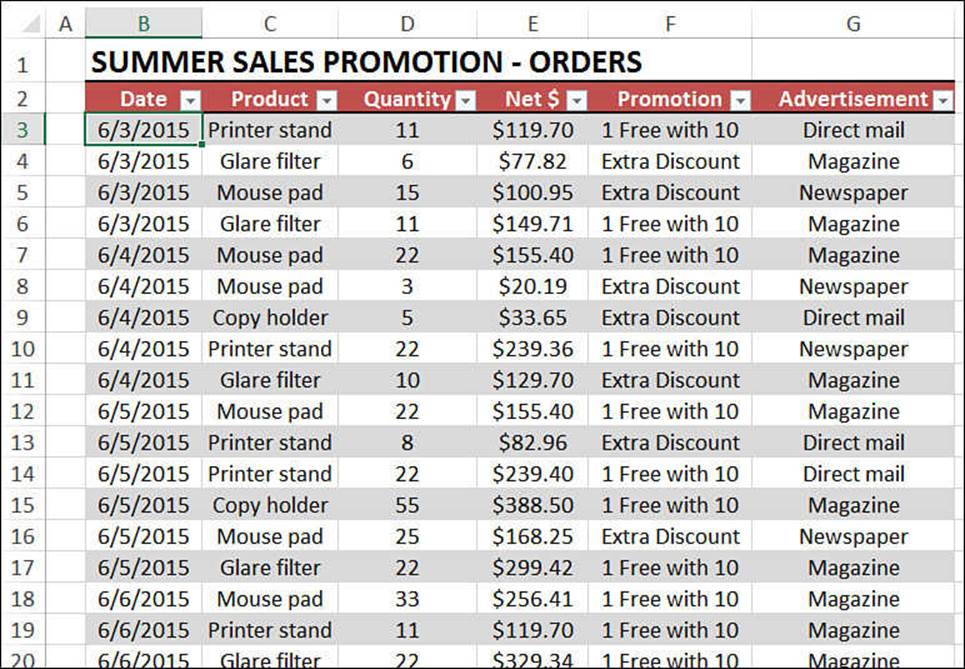
Figure 14.5 A table of orders to be summarized with a PivotTable.
Here are the steps to follow to summarize a table or range with a PivotTable:
1. Click a cell inside the table or range.
2. Determine how to proceed next, based on the type of data you want to summarize:
• If you’re working with a table, select Design, Summarize with PivotTable.
• If you’re working with a table or range, select Insert, PivotTable.
3. In the Create PivotTable dialog box that appears (see Figure 14.6), you should already see either the table name or the range address in the Select a Table or Range box. If not, enter or select the table name or range.
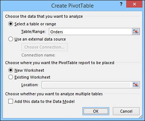
Figure 14.6 Use the Create PivotTable dialog box to specify the table or range to use as the data source, as well as the location of the PivotTable.
4. Choose where you want the PivotTable report to appear:
• New Worksheet—Click this option (it’s selected by default) to have Excel create a new worksheet for the PivotTable.
• Existing Worksheet—Click this option and then use the Location range box to type or select the cell where you want the PivotTable to appear. (The cell you specify will be the upper-left cell of the PivotTable.)
5. Click OK. Excel creates the PivotTable skeleton and displays the PivotTable Field List pane as well as two PivotTable Tools tabs: Analyze and Design (see Figure 14.7).
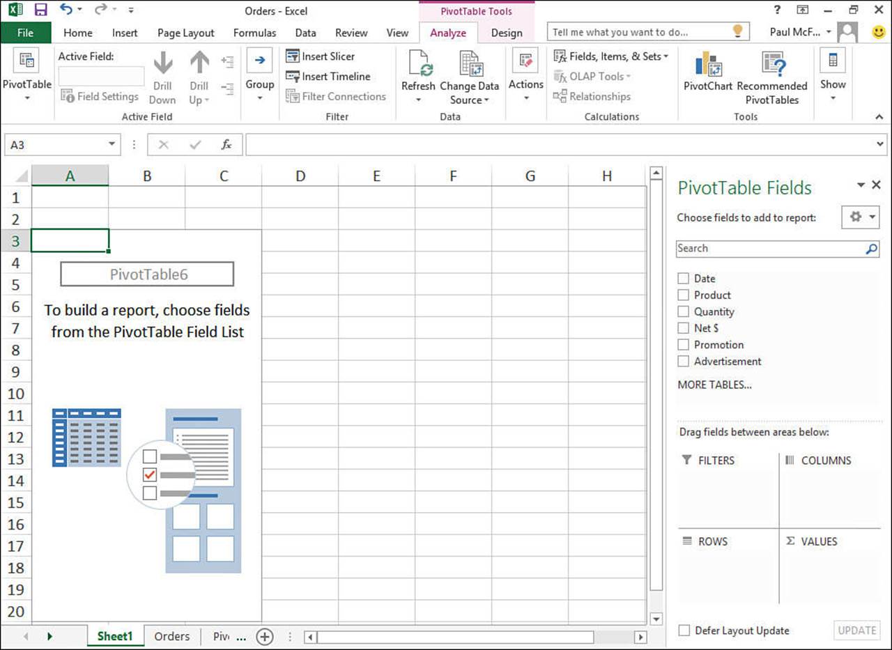
Figure 14.7 Excel starts off by creating a barebones PivotTable report.
6. Add a field that you want to appear in the report. Excel gives you two ways to do this:
• In the Choose Fields to Add to Report list, click to select the check box beside the field you want to add. If you select the check box of a numeric field, Excel adds it to the Values area; if you select the check box of a text field, Excel adds it to the Rows area.
• Click-and-drag the field and drop it inside the area where you want the field to appear.
Tip
If you want to use a field in the PivotTable’s column area, select its check box to add it to the Rows area, and then click-and-drag the field and drop it in the Columns area. You can also click-and-drag the field directly to the Columns area.
Tip
If you’re using an exceptionally large data source, it may take Excel a long time to update the PivotTable as you add each field. In this case, click to select the Defer Layout Update check box, which tells Excel not to update the PivotTable as you add each field. When you’re ready to see the current PivotTable layout, click Update.
7. Repeat step 6 to add all the fields you want included in the report. As you add each field, Excel updates the PivotTable report. For example, Figure 14.8 shows the report with the Quantity and Product fields added.
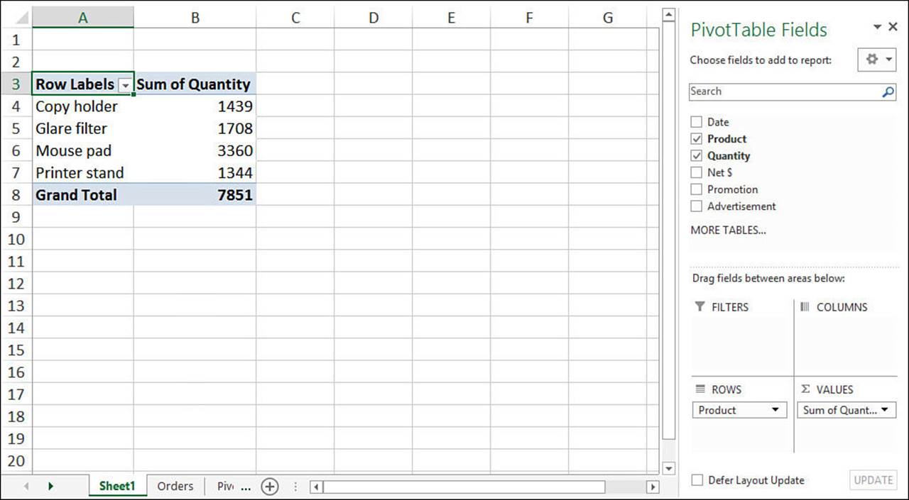
Figure 14.8 The PivotTable report with Product added to the Rows area and Quantity added to the Values area.
Building a PivotTable from an External Database
Excel can still put together a PivotTable even if your source data exists in an external database (for example, an Access or SQL Server database). If you have existing data connections on your system, you can use one of them as the data source. Otherwise, you can create a new connection on the fly. Here are the steps to follow:
1. Select Insert, PivotTable. Excel displays the Create PivotTable dialog box.
2. Select Use an External Data Source.
3. Click Choose Connection. Excel displays the Existing Connections dialog box.
4. If you see the connection you want to use, click it and skip to step 10. Otherwise, click Browse for More to open the Select Data Source dialog box.
5. Click New Source to launch the Data Connection Wizard.
6. Click the type of data source you want and then click Next.
7. Specify the data source. (How you do this depends on the type of data. For SQL Server, you specify the Server Name and Log On Credentials; for an ODBC data source, such as an Access database, you specify the database file.)
8. Select the database and table you want to use and then click Next.
9. Click Finish to complete the Data Connection Wizard.
10. To complete the PivotTable, follow steps 3 through 7 from the previous section.
Note
You can also create a PivotTable directly when you import data from an external source. In the Data tab’s Get External Data group, select the type of data source you want to import and then follow the instructions on the screen. When you get to the Import Data dialog box, select the PivotTable Report option and then click OK.
Working with and Customizing a PivotTable
As I mentioned earlier, I’m going to concentrate in this chapter on PivotTable formulas and calculations. To that end, the list that follows takes you quickly through a few basic Pivot Table chores that you should know. Note that in almost all cases, you first need to click inside the PivotTable to enable the Analyze and Design tabs. Here’s the list:
![]() Selecting an entire PivotTable—Select Analyze, Actions, Select, Entire PivotTable.
Selecting an entire PivotTable—Select Analyze, Actions, Select, Entire PivotTable.
![]() Selecting PivotTable items—Select the entire PivotTable and then select Analyze, Actions, Select. In the list, click the PivotTable element you want to select: Labels and Values, Values, or Labels.
Selecting PivotTable items—Select the entire PivotTable and then select Analyze, Actions, Select. In the list, click the PivotTable element you want to select: Labels and Values, Values, or Labels.
![]() Formatting a PivotTable—Select the Design tab and then click a style in the PivotTable Styles gallery.
Formatting a PivotTable—Select the Design tab and then click a style in the PivotTable Styles gallery.
![]() Changing a PivotTable name—Select the Analyze tab and then edit the PivotTable Name text box that appears in the PivotTable group.
Changing a PivotTable name—Select the Analyze tab and then edit the PivotTable Name text box that appears in the PivotTable group.
![]() Sorting a PivotTable—Drop down the row or column header’s filter button and then click either Sort A to Z or Sort Z to A. (If the field contains dates, click Sort Oldest to Newest or Sort Newest to Oldest, instead.)
Sorting a PivotTable—Drop down the row or column header’s filter button and then click either Sort A to Z or Sort Z to A. (If the field contains dates, click Sort Oldest to Newest or Sort Newest to Oldest, instead.)
![]() Refreshing PivotTable data—Select the Analyze tab and then click the top half of the Refresh button.
Refreshing PivotTable data—Select the Analyze tab and then click the top half of the Refresh button.
![]() Filtering a PivotTable—Click-and-drag a field to the Filters area, drop down the filter list, and then click an item in the list.
Filtering a PivotTable—Click-and-drag a field to the Filters area, drop down the filter list, and then click an item in the list.
![]() Grouping PivotTable data by date or numeric data—Click the field, select Analyze, Group, Group Field to open the Grouping dialog box, and then click the grouping you want to use. For a date field, for example, you can group by months, quarters, or years.
Grouping PivotTable data by date or numeric data—Click the field, select Analyze, Group, Group Field to open the Grouping dialog box, and then click the grouping you want to use. For a date field, for example, you can group by months, quarters, or years.
![]() Grouping PivotTable data by field items—In the field, select each item you want to include in the group. Then select Analyze, Group, Group Selection.
Grouping PivotTable data by field items—In the field, select each item you want to include in the group. Then select Analyze, Group, Group Selection.
![]() Removing a field from a PivotTable—Click-and-drag the field from the PivotTable Field List pane and drop it outside the pane.
Removing a field from a PivotTable—Click-and-drag the field from the PivotTable Field List pane and drop it outside the pane.
![]() Clearing a PivotTable—Select Analyze, Actions, Clear, Clear All.
Clearing a PivotTable—Select Analyze, Actions, Clear, Clear All.
Working with PivotTable Subtotals
You’ve seen that Excel adds grand totals to a PivotTable for the row field and the column field. However, Excel also displays subtotals for the outer field of a PivotTable with multiple fields in the row or column area. For example, in Figure 14.9, you see two fields in the row area: Product (Copy holder, Glare filter, and so on) and Promotion (1 Free with 10 and Extra Discount). Product is the outer field, so Excel displays subtotals for that field.
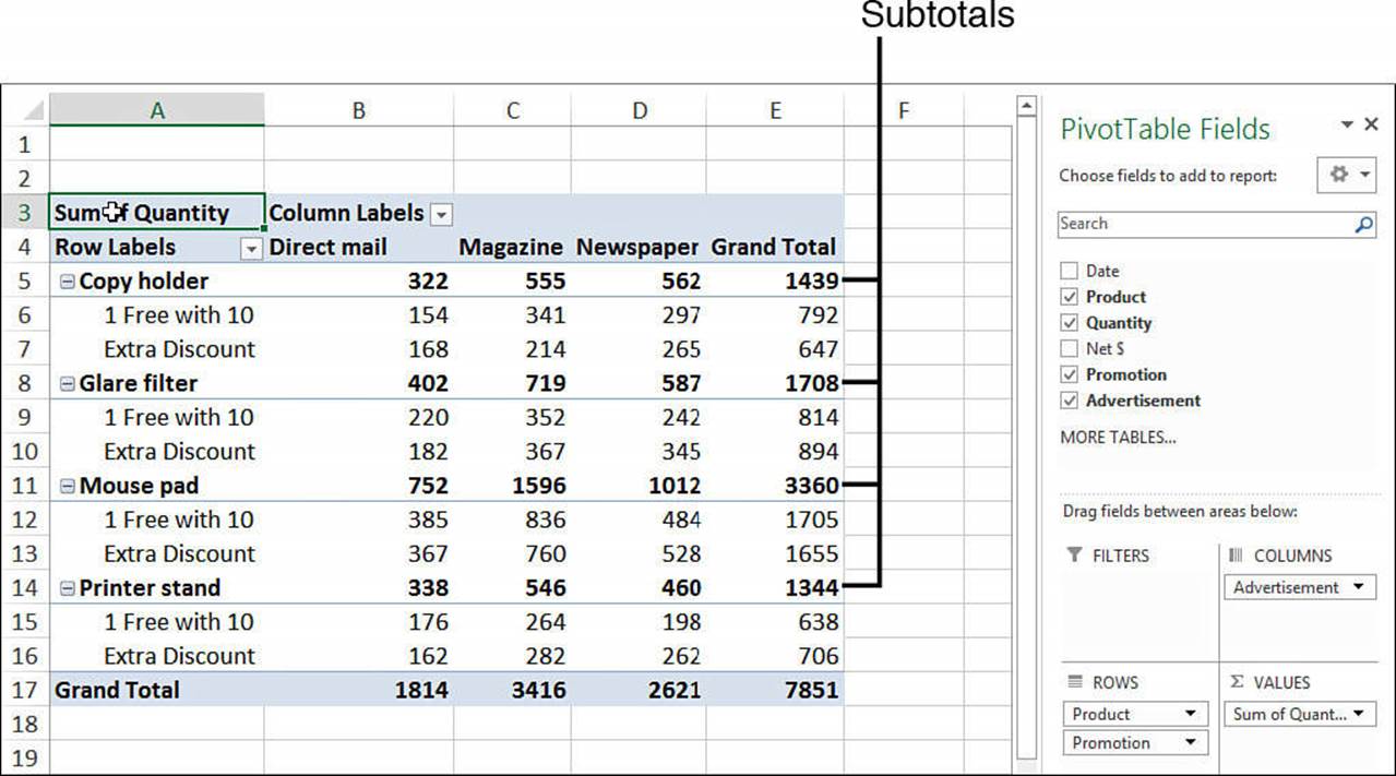
Figure 14.9 When you add multiple fields to the row or column area, Excel displays subtotals for the outer field.
The next few sections show you how to manipulate both the grand totals and the subtotals.
Hiding PivotTable Grand Totals
To remove grand totals from a PivotTable, follow these steps:
1. Select a cell inside the PivotTable.
2. Click the Design tab.
3. Select Grand Totals, Off for Rows and Columns. Excel removes the grand totals from the PivotTable.
Hiding PivotTable Subtotals
PivotTables with multiple row or column fields display subtotals for all fields except the innermost field (that is, the field closest to the data area). To remove these subtotals, follow these steps:
1. Select a cell in the field.
2. Click the Design tab.
3. Select Subtotals, Do Not Show Subtotals. Excel removes the subtotals from the PivotTable.
Customizing the Subtotal Calculation
The subtotal calculation that Excel applies to a field is the same calculation it uses for the data area. (See the next section for details on how to change the data field summary calculation.) You can, however, change this calculation, add extra calculations, and even add a subtotal for the innermost field. Click the field you want to work with, select Analyze, Active Field, Field Settings, and then use either of these methods:
![]() To change the subtotal calculation, click Custom in the Subtotals group, click one of the calculation functions (Sum, Count, Average, and so on) in the Select One or More Functions list, and then click OK.
To change the subtotal calculation, click Custom in the Subtotals group, click one of the calculation functions (Sum, Count, Average, and so on) in the Select One or More Functions list, and then click OK.
![]() To add extra subtotal calculations, click Custom in the Subtotals group, use the Select One or More Functions list to click each calculation function you want to add, and then click OK.
To add extra subtotal calculations, click Custom in the Subtotals group, use the Select One or More Functions list to click each calculation function you want to add, and then click OK.
Changing the Data Field Summary Calculation
By default, Excel uses a Sum function for calculating the data field summaries. Although Sum is the most common summary function used in PivotTables, it’s by no means the only one. In fact, Excel offers 11 summary functions, as outlined in Table 14.1.
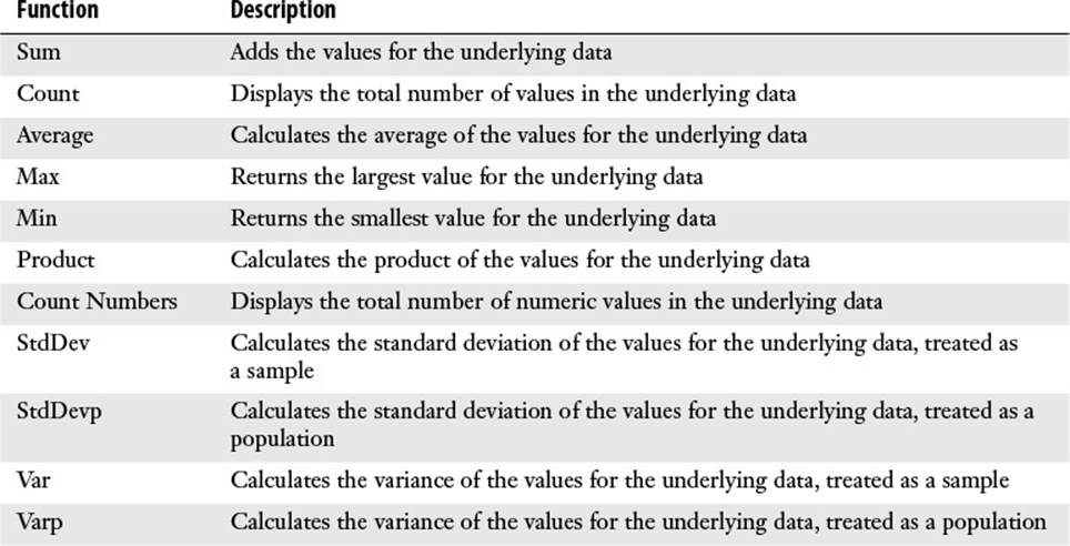
Table 14.1 Excel’s Data Field Summary Calculations
Follow these steps to change the data field summary calculation:
1. Right-click any cell inside the data field.
2. Select Summarize Values By. Excel displays a partial list of the available summary calculations.
3. If you see the calculation you want, click it and skip the rest of these steps; otherwise, click More Options to open the Value Field Settings dialog box.
4. Select the summary calculation you want to use.
5. Click OK. Excel changes the data field calculation.
Using a Difference Summary Calculation
When you analyze business data, it’s almost always useful to summarize the data as a whole: the sum of the units sold, the total number of orders, the average margin, and so on. For example, the PivotTable report shown in Figure 14.10 summarizes invoice data from a two-year period. For each customer in the row field, we see the total of all invoices broken down by the invoice date, which in this case has been grouped by year (2014 and 2015).
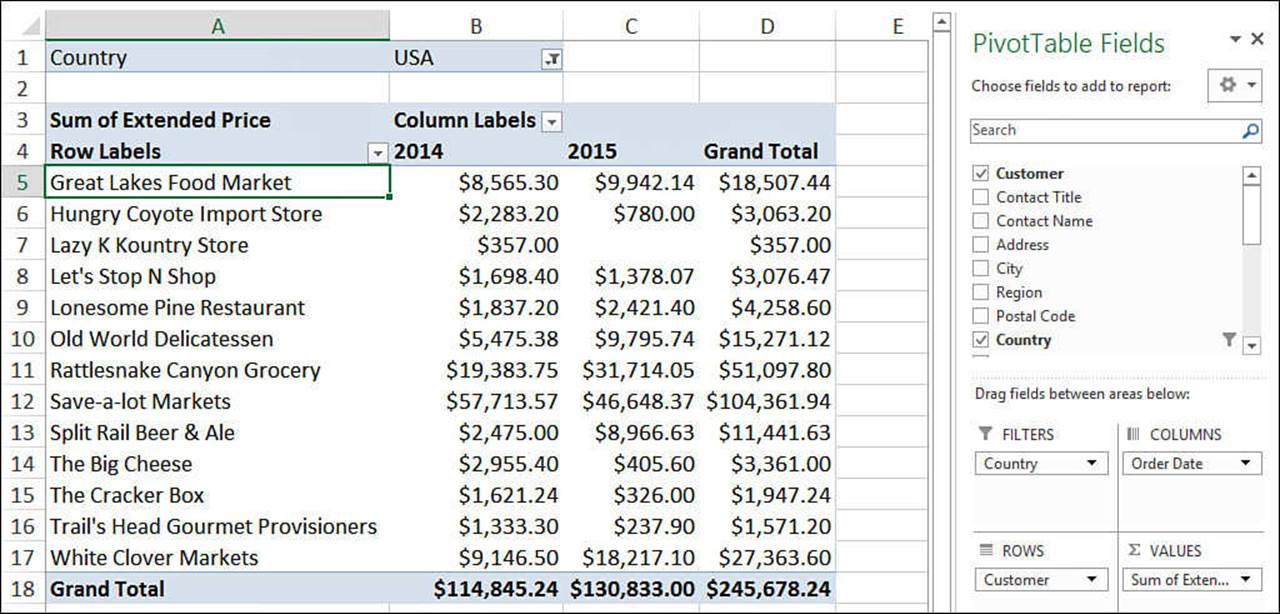
Figure 14.10 A PivotTable report showing customer invoice totals by year.
However, it’s also useful to compare one part of the data with another. In the PivotTable shown in Figure 14.10, for example, it would be valuable to compare each customer’s invoice totals in 2015 with those in 2014.
In Excel, you can perform this kind of analysis by using PivotTable difference calculations:
![]() Difference From—This difference calculation compares two numeric items and calculates the difference between them.
Difference From—This difference calculation compares two numeric items and calculates the difference between them.
![]() % Difference From—This difference calculation compares two numeric items and calculates the percentage difference between them.
% Difference From—This difference calculation compares two numeric items and calculates the percentage difference between them.
In each case, you must specify both a base field (the field in which you want Excel to perform the difference calculation) and the base item (the item in the base field that you want to use as the basis of the difference calculation). In the PivotTable shown in Figure 14.10, for example, Order Date would be the base field, and 2014 would be the base item.
Here are the steps to follow to set up a difference calculation:
1. Right-click any cell inside the data field.
2. Select Show Values As and then click either Difference From or % Difference From. Excel displays the Show Values As dialog box.
3. In the Base Field list, click the field you want to use as the base field.
4. In the Base Item list, click the item you want to use as the base item.
5. Click OK. Excel updates the PivotTable with the difference calculation.
Figure 14.11 shows both the completed Show Values As dialog box and the updated PivotTable with the Difference From calculation applied to the report from Figure 14.10.
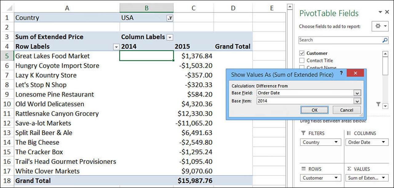
Figure 14.11 The PivotTable report from Figure 14.10 with a Difference From calculation applied.
Toggling the Difference Calculation
Here’s a VBA macro that toggles the PivotTable report in Figure 14.11 between a Difference From calculation and a % Difference From calculation:
Sub ToggleDifferenceCalculations()
' Work with the first data field
With Selection.PivotTable.DataFields(1)
' Is the calculation currently Difference From?
If .Calculation = xlDifferenceFrom Then
' If so, change it to % Difference From
.Calculation = xlPercentDifferenceFrom
.BaseField = "Order Date"
.BaseItem = "2014"
.NumberFormat = "0.00%"
Else
' If not, change it to Difference From
.Calculation = xlDifferenceFrom
.BaseField = "Order Date"
.BaseItem = "2014"
.NumberFormat = "$#,##0.00"
End If
End With
End Sub
Using a Percentage Summary Calculation
When you need to compare the results that appear in a PivotTable report, just looking at the basic summary calculations isn’t always useful. For example, consider the PivotTable report in Figure 14.12, which shows the total invoices put through by various sales reps, broken down by quarter. In the fourth quarter, Margaret Peacock put through $64,429, whereas Robert King put through only $16,951. You can’t say that the first rep is (roughly) four times as good a salesperson as the second rep because their territories or customers might be completely different. A better way to analyze these numbers would be to compare the fourth quarter figures with some base value, such as the first quarter total. The numbers are down in both cases, but again the raw differences won’t tell you much. What you need to do is calculate the percentage differences and then compare them with the percentage difference in the Grand Total.
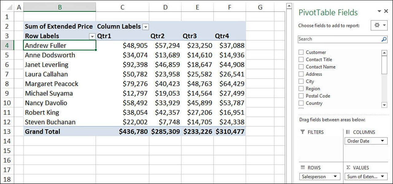
Figure 14.12 A PivotTable report showing sales rep invoice totals by quarter.
Similarly, knowing the raw invoice totals for each rep in a given quarter gives you only the most general idea of how the reps did with respect to each other. If you really want to compare them, you need to convert those totals into percentages of the quarterly grand total.
When you want to use percentages in your data analysis, you can use Excel’s percentage calculations to view data items as a percentage of some other item or as a percentage of the total in the current row, column, or the entire PivotTable. Excel offers the following percentage calculations:
![]() % Of—This calculation returns the percentage of each value with respect to a selected base item. If you use this calculation, you must also select a base field and a base item upon which Excel will calculate the percentages.
% Of—This calculation returns the percentage of each value with respect to a selected base item. If you use this calculation, you must also select a base field and a base item upon which Excel will calculate the percentages.
![]() % of Row Total—This calculation returns the percentage that each value in a row represents with respect to the Grand Total for that row.
% of Row Total—This calculation returns the percentage that each value in a row represents with respect to the Grand Total for that row.
![]() % of Column Total—This calculation returns the percentage that each value in a column represents with respect to the Grand Total for that column.
% of Column Total—This calculation returns the percentage that each value in a column represents with respect to the Grand Total for that column.
![]() % of Parent Row Total—If you have multiple fields in the row area, this calculation returns the percentage that each value in an inner row represents with respect to the total of the parent item in the outer row. (This calculation also returns the percentage that each value in the outer row represents with respect to the Grand Total.)
% of Parent Row Total—If you have multiple fields in the row area, this calculation returns the percentage that each value in an inner row represents with respect to the total of the parent item in the outer row. (This calculation also returns the percentage that each value in the outer row represents with respect to the Grand Total.)
![]() % of Parent Column Total—If you have multiple fields in the column area, this calculation returns the percentage that each value in an inner column represents with respect to the total of the parent item in the outer column. (This calculation also returns the percentage that each value in the outer column represents with respect to the Grand Total.)
% of Parent Column Total—If you have multiple fields in the column area, this calculation returns the percentage that each value in an inner column represents with respect to the total of the parent item in the outer column. (This calculation also returns the percentage that each value in the outer column represents with respect to the Grand Total.)
![]() % of Parent Total—If you have multiple fields in the row or column area, this calculation returns the percentage of each value with respect to a selected base field in the outer row or column. If you use this calculation, you must also select a base field upon which Excel will calculate the percentages.
% of Parent Total—If you have multiple fields in the row or column area, this calculation returns the percentage of each value with respect to a selected base field in the outer row or column. If you use this calculation, you must also select a base field upon which Excel will calculate the percentages.
![]() % of Grand Total—This calculation returns the percentage that each value in the PivotTable represents with respect to the Grand Total of the entire PivotTable.
% of Grand Total—This calculation returns the percentage that each value in the PivotTable represents with respect to the Grand Total of the entire PivotTable.
Here are the steps to follow to set up a difference calculation:
1. Right-click any cell inside the data field.
2. Select Show Values As and then click the percentage calculation you want to use. Excel displays the Show Values As dialog box.
3. If you chose either % Of or % of Parent Total, use the Base Field list to click the field you want to use as the base field.
4. If you clicked % Of, use the Base Item list to click the item you want to use as the base item.
5. Click OK. Excel updates the PivotTable with the percentage calculation.
Figure 14.13 shows both the completed Show Values As dialog box and the updated PivotTable with the % Of calculation applied to the report from Figure 14.12.
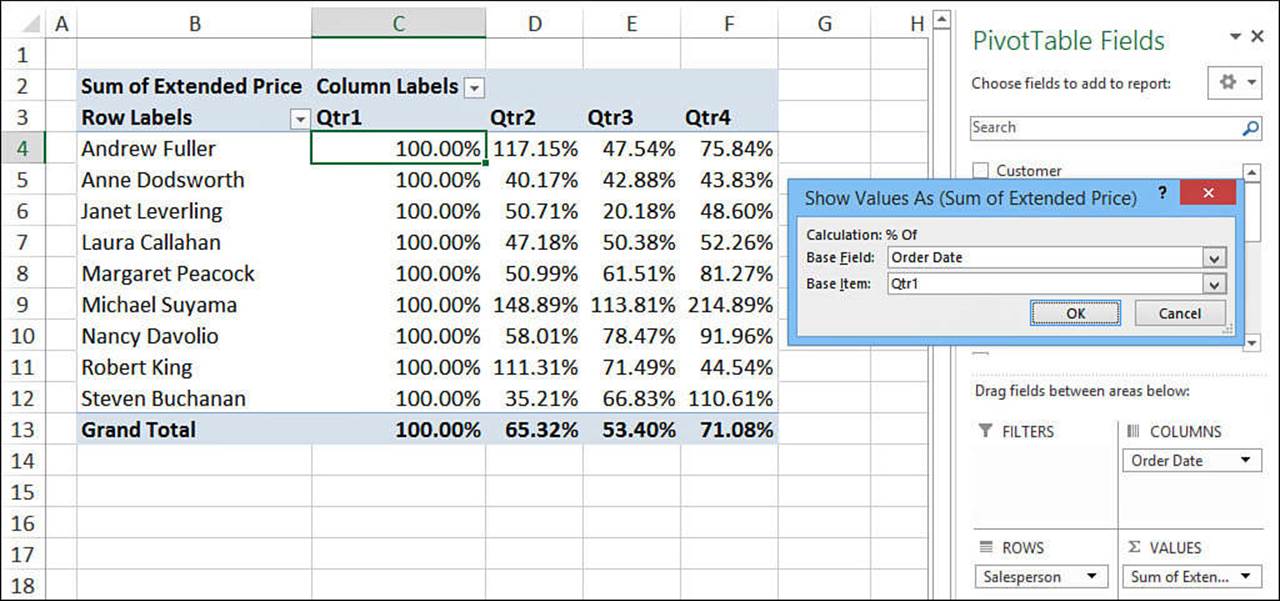
Figure 14.13 The PivotTable report from Figure 14.12 with a % Of calculation applied.
Tip
If you want to use a VBA macro to set the percentage calculation for a data field, set the PivotField object’s Calculation property to one of the following constants: xlPercentOf, xlPercentOfRow, xlPercentOfColumn, or xlPercentOfTotal.
When you switch back to Normal in the Show Values As list, Excel formats the data field as General, so you lose any numeric formatting you had applied. You can restore the numeric format by clicking inside the data field, choosing Analyze, Active Field, Field Settings, clicking Number Format, and then choosing the format in the Format Cells dialog box. Alternatively, you can use a macro that resets the NumberFormat property. Here’s an example:
Sub ReapplyCurrencyFormat()
With Selection.PivotTable.DataFields(1)
.NumberFormat = "$#,##0.00"
End With
End Sub
Using a Running Total Summary Calculation
When you set up a budget, it’s common to have sales targets not only for each month but also cumulative targets as the fiscal year progresses. For example, you might have sales targets for the first month and the second month and also for the two-month total. You’d also have cumulative targets for three months, four months, and so on. Cumulative sums such as these are known as running totals, and they can be valuable in analysis. For example, if you find that you’re running behind budget cumulatively at the six-month mark, you can make adjustments to process, marketing plans, customer incentives, and so on.
Excel PivotTable reports come with a Running Total summary calculation that you can use for this kind of analysis. Note that the running total is always applied to a base field, which is the field on which you want to base the accumulation. This is almost always a date field, but you can use other field types, as appropriate.
Here are the steps to follow to set up a running total calculation:
1. Right-click any cell inside the data field.
2. Select Show Values As, Running Total In. Excel displays the Show Values As dialog box.
3. Use the Base Field list to click the field you want to use as the base field.
4. Click OK. Excel updates the PivotTable with the running total calculation.
Figure 14.14 shows both the completed Show Values As dialog box and a PivotTable with the Running Total In calculation applied to the Order Date field (grouped by month).
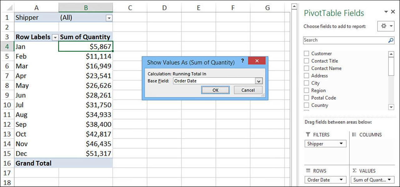
Figure 14.14 The PivotTable report with a running total calculation.
Tip
If you use many of these extra summary calculations, you might find yourself constantly returning the No Calculation value in the Show Values As menu. That requires a few mouse clicks, so it can be a hassle to repeat the procedure frequently. You can save time by creating a VBA macro that resets the PivotTable to Normal by setting the Calculation property to xlNoAdditionalCalculation. Here’s an example:
Sub ResetCalculationToNormal()
With Selection.PivotTable.DataFields(1)
.Calculation = xlNoAdditionalCalculation
End With
End Sub
Using an Index Summary Calculation
A PivotTable is great for reducing a large amount of relatively incomprehensible data into a compact, more easily grasped summary report. As you’ve seen in the past few sections, however, a standard summary calculation doesn’t always provide you with the best analysis of the data.
Another good example of this is trying to determine the relative importance of the results in the data field. For example, consider the PivotTable report shown in Figure 14.15. This report shows the unit sales of four items (copy holder, glare filter, mouse pad, and printer stand), broken down by the type of advertisement the customer responded to (direct mail, magazine, and newspaper).
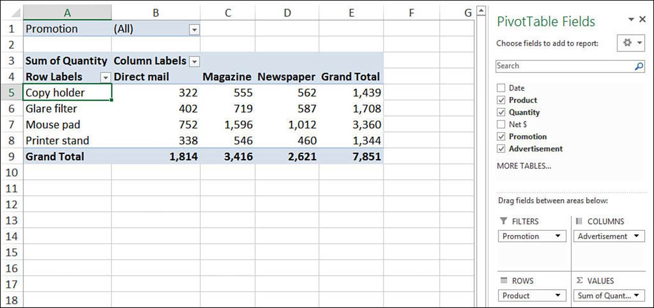
Figure 14.15 A PivotTable report showing unit sales of products broken down by advertisement.
You can see, for example, that 1,012 mouse pads were sold via the newspaper ad (the second-highest number in the report), but only 562 copy holders were sold through the newspaper (one of the lower numbers in the report). Does this mean that you should only sell mouse pads in newspaper ads? That is, is the mouse pad/newspaper combination somehow more “important” than the copy holder/newspaper combination?
You might think the answer is yes to both questions in the previous paragraph, but that’s not necessarily the case. To get an accurate answer, you’d need to take into account the total number of mouse pads sold, the total number of copy holders sold, the total number of units sold through the newspaper, and the number of units overall. This is a complicated bit of business, to be sure, but each PivotTable report has an Index calculation that handles it for you automatically. The Index calculation returns the weighted average of each cell in the PivotTable data field, using the following formula:
(Cell Value) * (Grand Total) / (Row Total) * (Column Total)
In the Index calculation results, the higher the value, the more important the cell is in the overall results. Here are the steps to follow to set up an Index calculation:
1. Right-click any cell inside the data field.
2. Select Summarize Values By and then click the summary calculation you want to use.
3. Right-click any cell inside the data field.
4. Select Show Values As, Index. Excel updates the PivotTable with the index summary calculation.
Figure 14.16 shows the updated PivotTable with the Index applied to the report from Figure 14.15. As you can see, the mouse pad/newspaper combination scored an index of only 0.90 (the second-lowest value), whereas the copy holder/newspaper combination scored 1.17 (the highest value).
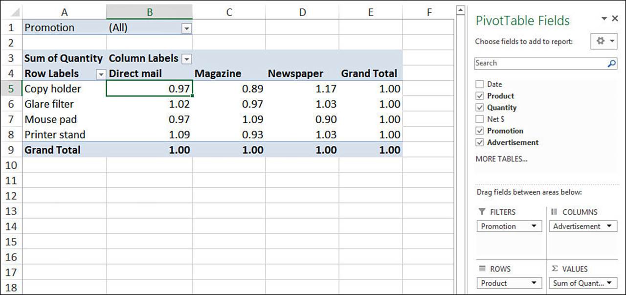
Figure 14.16 The PivotTable report from Figure 14.15 with an Index calculation applied.
Creating Custom PivotTable Calculations
Excel’s 11 built-in summary functions enable you to create powerful and useful PivotTable reports, but they don’t cover every data analysis possibility. For example, suppose you have a PivotTable report that summarizes invoice totals by sales rep using the Sum function. That’s useful, but you might also want to pay out a bonus to those reps whose total sales exceed some threshold. You could use the GETPIVOTDATA() function to create regular worksheet formulas to calculate whether bonuses should be paid and how much they should be (assuming each bonus is a percentage of the total sales).
![]() For the details on the GETPIVOTDATA() function, see “Using PivotTable Results in a Worksheet Formula,” p. 347.
For the details on the GETPIVOTDATA() function, see “Using PivotTable Results in a Worksheet Formula,” p. 347.
However, this isn’t very convenient. If you add sales reps, you need to add formulas; if you remove sales reps, existing formulas generate errors. And, in any case, one of the points of generating a PivotTable report is to perform fewer worksheet calculations, not more.
The solution in this case is to take advantage of Excel’s calculated field feature. A calculated field is a new data field based on a custom formula. For example, if your invoice’s PivotTable has an Extended Price field and you want to award a 5% bonus to those reps who did at least $75,000 worth of business, you’d create a calculated field based on the following formula:
=IF('Extended Price' >= 75000, 'Extended Price' * 0.05, 0)
Note
When you reference a field in your formula, Excel interprets this reference as the sum of that field’s values. For example, if you include the logical expression 'Extended Price' >= 75000 in a calculated field formula, Excel interprets this as Sum of 'Extended Price' >= 75000. That is, it adds the Extended Price field and then compares it with 75000.
A slightly different PivotTable problem is when a field you’re using for the row or column labels doesn’t contain an item you need. For example, suppose your products are organized into various categories: Beverages, Condiments, Confections, Dairy Products, and so on. Suppose further that these categories are grouped into several divisions: Beverages and Condiments in Division A, Confections and Dairy Products in Division B, and so on. If the source data doesn’t have a Division field, how do you see PivotTable results that apply to the divisions?
One solution is to create groups for each division. (That is, select the categories for one division, select Analyze, Group Selection, and repeat for the other divisions.) That works, but Excel gives you a second solution: Use calculated items. A calculated item is a new item in a row or column where the item’s values are generated by a custom formula. For example, you could create a new item named Division A that is based on the following formula:
=Beverages + Condiments
Before getting to the details of creating calculated fields and items, you should know that Excel imposes a few restrictions on them. Here’s a summary:
![]() You can’t use a cell reference, range address, or range name as an operand in a custom calculation formula.
You can’t use a cell reference, range address, or range name as an operand in a custom calculation formula.
![]() You can’t use the PivotTable’s subtotals, row totals, column totals, or Grand Total as an operand in a custom calculation formula.
You can’t use the PivotTable’s subtotals, row totals, column totals, or Grand Total as an operand in a custom calculation formula.
![]() In a calculated field, Excel defaults to a Sum calculation when you reference another field in your custom formula. However, this can cause problems. For example, suppose your invoice table has Unit Price and Quantity fields. You might think that you can create a calculated field that returns the invoice totals with the following formula:
In a calculated field, Excel defaults to a Sum calculation when you reference another field in your custom formula. However, this can cause problems. For example, suppose your invoice table has Unit Price and Quantity fields. You might think that you can create a calculated field that returns the invoice totals with the following formula:
=Unit Price * Quantity
This won’t work, however, because Excel treats the Unit Price operand as Sum of Unit Price, and it doesn’t make sense to “add” the prices together.
![]() For a calculated item, the custom formula can’t reference items from any field except the one in which the calculated item resides.
For a calculated item, the custom formula can’t reference items from any field except the one in which the calculated item resides.
![]() You can’t create a calculated item in a PivotTable that has at least one grouped field. You must ungroup all the PivotTable fields before you can create a calculated item.
You can’t create a calculated item in a PivotTable that has at least one grouped field. You must ungroup all the PivotTable fields before you can create a calculated item.
![]() You can’t use a calculated item as a filter.
You can’t use a calculated item as a filter.
![]() You can’t insert a calculated item into a PivotTable in which a field has been used more than once.
You can’t insert a calculated item into a PivotTable in which a field has been used more than once.
![]() You can’t insert a calculated item into a PivotTable that uses the Average, StdDev, StdDevp, Var, or Varp summary calculations.
You can’t insert a calculated item into a PivotTable that uses the Average, StdDev, StdDevp, Var, or Varp summary calculations.
Creating a Calculated Field
Here are the steps to follow to insert a calculated field into a PivotTable data area:
1. Click any cell in the PivotTable’s data area.
2. Select Analyze, open the Fields, Items, & Sets list, and then select Calculated Field. Excel displays the Insert Calculated Field dialog box.
3. Use the Name text box to enter a name for the calculated field.
4. Use the Formula text box to enter the formula you want to use for the calculated field.
Note
If you need to use a field name in the formula, position the cursor where you want the field name to appear, click the field name in the Fields list, and then click Insert Field.
5. Click Add.
6. Click OK. Excel inserts the calculated field into the PivotTable.
Figure 14.17 shows a completed version of the Insert Calculated Field dialog box, as well as the resulting Bonus field in the PivotTable. Here’s the full formula that appears in the Formula text box:
=IF('Extended Price' >= 75000, 'Extended Price' * 0.05, 0)
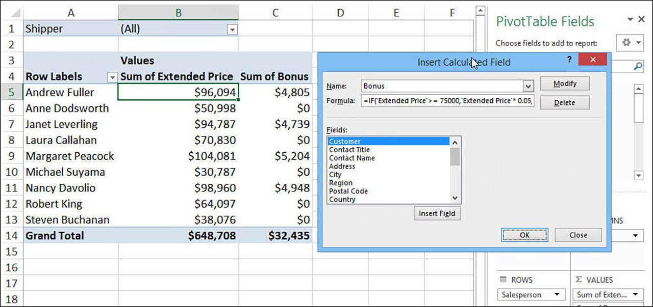
Figure 14.17 A PivotTable report with a Bonus calculated field.
Note
If you need to make changes to a calculated field, click any cell in the PivotTable’s data area, select Analyze, open the Fields, Items, & Sets list, select Calculated Field, and then use the Name list to select the calculated field you want to work with. Make your changes to the formula, click Modify, and then click OK.
Caution
In Figure 14.17, notice that the Grand Total row also includes a total for the Bonus field. Notice, too, that the total displayed is incorrect! This is almost always the case with calculated fields. The problem is that Excel doesn’t derive the calculated field’s Grand Total by adding up the field’s values. Instead, Excel applies the calculated field’s formula to the Grand Total of whatever field you reference in the formula. For example, in the logical expression 'Extended Price' >= 75000, Excel uses the Grand Total of the Extended Price field. Because this is definitely more than 75,000, Excel calculates the “bonus” of 5%, which is the value that appears in the Bonus field’s Grand Total.
Creating a Calculated Item
Here are the steps to follow to insert a calculated item into a PivotTable’s row or column area:
1. Click any cell in the row or column field to which you want to add the item.
2. Select Analyze, open the Fields, Items, & Sets list, and then select Calculated Item. Excel displays the Insert Calculated Item in “Field” dialog box (where Field is the name of the field you’re working with).
3. Use the Name text box to enter a name for the calculated item.
4. Use the Formula text box to enter the formula you want to use for the calculated item.
Note
To add a field name to the formula, position the cursor where you want the field name to appear, click the field name in the Fields list, and then click Insert Field. To add a field item to the formula, position the cursor where you want the item name to appear, click the field in the Fields list, click the item in the Items list, and then click Insert Item.
5. Click Add.
6. Repeat steps 3-5 to add other calculated items to the field.
7. Click OK. Excel inserts the calculated item or items into the row or column field.
Figure 14.18 shows a completed version of the Insert Calculated Item in “Field” dialog box, as well as three items added to the Category row field:
Division A: =Beverage + Condiments
Division B: =Confections + 'Dairy Products'
Division C: ='Grains/Cereals' + 'Meat/Poultry' + Produce + Seafood
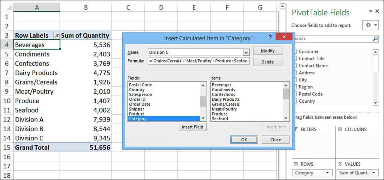
Figure 14.18 A PivotTable report with three calculated items added to the Category row field.
Note
To make changes to a calculated item, click any cell in the field that contains the item, select Analyze, open the Fields, Items, & Sets list, select Calculated Item, and then use the Name list to select the calculated item you want to work with. Make your changes to the formula, click Modify, and then click OK.
Caution
When you insert an item into a field, Excel remembers that item. (Technically, it becomes part of the data source’s pivot cache.) If you then insert the same field into another PivotTable based on the same data source, Excel also includes the calculated items in the new PivotTable. If you don’t want the calculated items to appear in the new PivotTable report, drop down the field’s menu and deselect the check box beside each calculated item.
Using PivotTable Results in a Worksheet Formula
What do you do when you need to include a PivotTable result in a regular worksheet formula? At first, you might be tempted just to include a reference to the appropriate cell in the PivotTable’s data area. However, that works only if your PivotTable is static and never changes. In the vast majority of cases, the reference won’t work because the addresses of the report values change as you pivot, filter, group, and refresh the PivotTable.
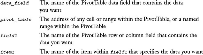
If you want to include a PivotTable result in a formula and you want that result to remain accurate even as you manipulate the PivotTable, use Excel’s GETPIVOTDATA() function. This function uses the data field, PivotTable location, and one or more (row or column) field/item pairs that specify the exact value you want to use. Here’s the syntax:
GETPIVOTDATA(data_field, pivot_table[, field1, item1]...])
Note that you always enter the fieldn and itemn arguments as a pair. If you don’t include any field/item pairs, GETPIVOTDATA() returns the PivotTable Grand Total. You can enter up to 126 field/item pairs. This might make GETPIVOTDATA() seem like more work than it’s worth, but the good news is that you’ll rarely have to enter the GETPIVOTDATA() function by hand. By default, Excel is configured to generate the appropriate GETPIVOTDATA() syntax automatically. That is, you start your worksheet formula, and when you get to the part where you need the PivotTable value, just click the value. Excel then inserts the GETPIVOTDATA() function with the syntax that returns the value you want.
For example, in Figure 14.19, you can see that I started a worksheet formula in cell F5 and then clicked cell B5 in the PivotTable. Excel generated the GETPIVOTDATA() function shown.
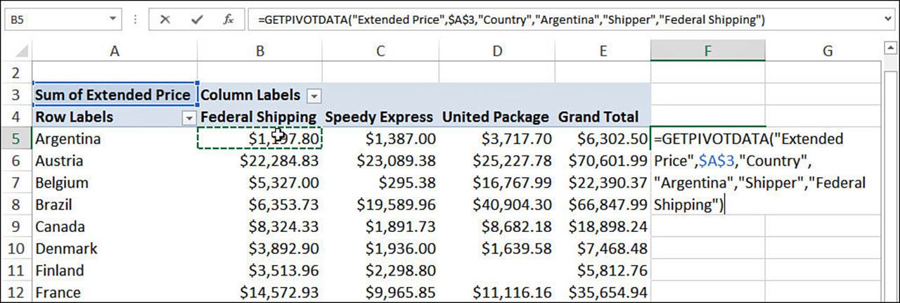
Figure 14.19 When you’re entering a worksheet formula, click a cell in a PivotTable’s data area, and Excel automatically generates the corresponding GETPIVOTDATA() function.
If Excel doesn’t generate the GETPIVOTDATA() function automatically, that feature may be turned off. Follow these steps to turn it back on:
1. Select File, Options to open the Excel Options dialog box.
2. Click Formulas.
3. Click to select the Use GetPivotData Functions for PivotTable References check box.
4. Click OK.
Tip
You can also use a VBA procedure to toggle automatic GETPIVOTDATA() functions on and off. Set the Application.GenerateGetPivotData property to True or False, as in the following macro:
Sub ToggleGenerateGetPivotData()
With Application
.GenerateGetPivotData = Not .GenerateGetPivotData
End With
End Sub
From Here
![]() To learn more about the IF() function used in this chapter, see “Using the IF() Function,” p. 164.
To learn more about the IF() function used in this chapter, see “Using the IF() Function,” p. 164.
![]() For a complete look at Excel tables, see Chapter 13, “Analyzing Data with Tables.”
For a complete look at Excel tables, see Chapter 13, “Analyzing Data with Tables.”
All materials on the site are licensed Creative Commons Attribution-Sharealike 3.0 Unported CC BY-SA 3.0 & GNU Free Documentation License (GFDL)
If you are the copyright holder of any material contained on our site and intend to remove it, please contact our site administrator for approval.
© 2016-2026 All site design rights belong to S.Y.A.