Excel® 2016 Formulas and Functions (2016)
Part II: Harnessing the Power of Functions
8. Working with Logical and Information Functions
In This Chapter
Adding Intelligence with Logical Functions
Getting Data with Information Functions
I mentioned in Chapter 6, “Understanding Functions,” that one of the advantages of using Excel’s worksheet functions is that they enable you to build formulas that perform actions that are simply not possible with the standard operators and operands.
This idea becomes readily apparent when you learn about functions that can add intelligence and knowledge—the two cornerstones of good business analysis—to your worksheet models. You get these via Excel’s logical and information functions, which I describe in detail in this chapter.
Adding Intelligence with Logical Functions
In the computer world, we very loosely define something as intelligent if it can perform tests on its environment and act in accordance with the results of those tests. However, computers are binary beasts, so “acting in accordance with the results of a test” means that the machine can do only one of two things. Still, even with this limited range of options, you’ll be amazed at how much intelligence you can bring to your worksheets. Your formulas will actually be able to test the values in cells and ranges and then return results based on those tests.
This is all done with Excel’s logical functions, which are designed to create decision-making formulas. For example, you can test cell contents to see whether they’re numbers or labels, or you can test formula results for errors. Table 8.1 summarizes Excel’s logical functions.
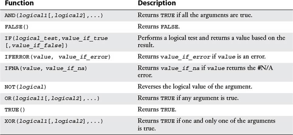
Table 8.1 Excel’s Logical Functions
![]() To learn about the IFERROR() and IFNA() functions, see “Handling Formula Errors with IFERROR(),” p. 118.
To learn about the IFERROR() and IFNA() functions, see “Handling Formula Errors with IFERROR(),” p. 118.
Using the IF() Function
I’m not exaggerating even the slightest when I tell you that the royal road to becoming an accomplished Excel formula builder involves mastering the IF() function. If you become comfortable wielding this function, a whole new world of formula prowess and convenience opens up to you. Yes, IF() is that powerful.
To help you master this crucial Excel feature, I’m going to spend a lot of time on it in this chapter. You’ll get copious examples that show you how to use it in real-world situations.
IF(): The Simplest Case
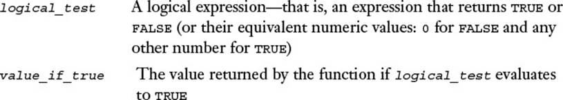
Let’s start with the simplest version of the IF() function:
IF(logical_test, value_if_true)
For example, consider the following formula:
=IF(A1 >= 1000, "It's big!")
The logical expression A1 >= 1000 is used as the test. Let’s say you enter this formula in cell B1. If the logical expression proves to be true (that is, if the value in cell A1 is greater than or equal to 1,000), the function returns the string It's big!, and that’s the value you see in cell B1. (If A1 is less than 1,000, you see the value FALSE in cell B1 instead.)
Another common use for the simple IF() test is to flag values that meet a specific condition. For example, suppose you have a worksheet that shows the percentage increase or decrease in the sales of a long list of products. It would be useful to be able to flag just those products that had a sales decrease. A basic formula for doing this would look something like this:
=IF(cell < 0, flag)
Here, cell is the cell you want to test, and flag is some text that you use to point out a negative value. Here’s an example:
=IF(B2 < 0, "<<<<<")
A slightly more sophisticated version of this formula would vary the flag, depending on the negative value. That is, the larger the negative number, the more less-than signs (in this case) the formula would display. This can be done using the REPT() function, discussed in Chapter 7, “Working with Text Functions”:
REPT("<", B2 * -100)
![]() For the details on the REPT() function, see “The REPT() Function: Repeating a Character or String,” p. 150.
For the details on the REPT() function, see “The REPT() Function: Repeating a Character or String,” p. 150.
This expression multiplies the percentage value by -100 and then uses the result as the number of times the less-than sign is repeated. Here’s the revised IF() formula:
=IF(B2 < 0, REPT("<", B2 * -100))
Figure 8.1 shows how it works in practice.
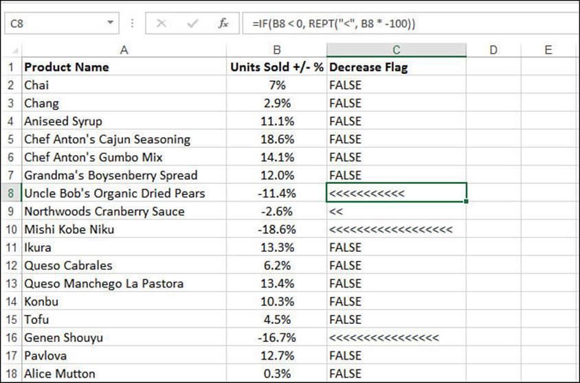
Figure 8.1 This worksheet uses the IF() function to test for negative values and then uses REPT() to display a flag for those values.
Note
You can download this chapter’s sample workbooks at www.mcfedries.com/books/book.php?title=excel-2016-formulas-and-functions.
Handling a FALSE Result
As you can see in Figure 8.1, if the result of the IF() condition calculates to FALSE, the function returns FALSE as its result. That’s not inherently bad, but the worksheet would look tidier (and, hence, be more useful) if the formula returned, say, the null string ("") instead.
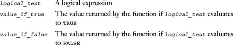
To do this, you need to use the full IF() function syntax:
IF(logical_test, value_if_true, value_if_false)
For example, consider the following formula:
=IF(A1 >= 1000, "It's big!", "It's not big!")
This time, if cell A1 contains a value that’s less than 1,000, the formula returns the string It's not big!.
For the negative value flag example, use the following revised version of the formula to return no value if the cell contains a nonnegative number:
=IF(B2 < 0, REPT("<", B2 * -100), "")
As you can see in Figure 8.2, the resulting worksheet looks much tidier than the first version.
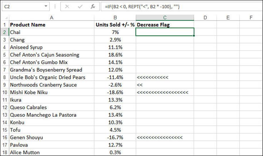
Figure 8.2 This worksheet uses the full IF() syntax to return no value if the cell being tested contains a nonnegative number.
Avoiding Division by Zero
As you saw in Chapter 5, “Troubleshooting Formulas,” Excel displays the #DIV/0! error if a formula tries to divide a quantity by zero. To avoid this error, you can use IF() to test the divisor and ensure that it’s nonzero before performing division.
![]() To learn about the #DIV/0! error, see “#DIV/0!,” p. 112.
To learn about the #DIV/0! error, see “#DIV/0!,” p. 112.
For example, the basic equation for calculating gross margin is (Sales - Expenses)/Sales. To make sure that Sales isn’t zero, use the following formula (assuming that you have cells named Sales and Expenses that contain the appropriate values):
=IF(Sales <> 0, (Sales - Expenses)/Sales, "Sales are zero!")
If the logical expression Sales <> 0 is true, that means Sales is nonzero, so the gross margin calculation can proceed. If Sales <> 0 is false, the Sales value is 0, so the message Sales are zero! is displayed instead.
Performing Multiple Logical Tests
The capability to perform a logical test on a cell is a powerful weapon indeed. You’ll find endless uses for the basic IF() function in your everyday worksheets. The problem, however, is that the everyday world often presents us with situations that are more complicated than can be handled in a basic IF() function’s logical expression. It’s often the case that you have to test two or more conditions before you can make a decision.
To handle these more complex scenarios, Excel offers several techniques for performing two or more logical tests: nested IF() functions, the AND() function, and the OR() function. You’ll learn about these techniques over the next few sections.
Nested IF() Functions
When building models using IF(), it’s common to come upon a second fork in the road when evaluating either the value_if_true or value_if_false argument.
For example, consider the variation of our formula that outputs a description based on the value in cell A1:
=IF(A1 > 1000, "Big!", "Not big")
What if you want to return a different string for values greater than, say, 10,000? In other words, if the condition A1 > 1000 proves to be true, you want to run another test that checks to see whether A1 > 10000. You can handle this scenario by nesting a second IF() function inside the first as the value_if_true argument:
=IF(A1 > 1000, IF(A1 > 10000, "Really big!!", "Big!"), "Not big")
If A1 > 1000 returns TRUE, the formula evaluates the nested IF(), which returns Really big!! if A1 > 10000 is TRUE and returns Big! if it’s FALSE; if A1 > 1000 returns FALSE, the formula returns Not big.
Note, too, that you can nest the IF() function in the value_if_false argument. For example, if you want to return the description Small for a cell value less than 100, you use this version of the formula:
=IF(A1 > 1000, "Big!", IF(A1 < 100, "Small", "Not big"))
Calculating Tiered Bonuses
A good time to use nested IF() functions arises when you need to calculate a tiered payment or charge. That is, if a certain value is X, you want one result; if the value is Y, you want a second result; and if the value is Z, you want a third result.
For example, suppose you want to calculate tiered bonuses for a sales team as follows:
![]() If the salesperson did not meet the sales target, no bonus is given.
If the salesperson did not meet the sales target, no bonus is given.
![]() If the salesperson exceeded the sales target by less than 10%, a bonus of $1,000 is awarded.
If the salesperson exceeded the sales target by less than 10%, a bonus of $1,000 is awarded.
![]() If the salesperson exceeded the sales target by 10% or more, a bonus of $10,000 is awarded.
If the salesperson exceeded the sales target by 10% or more, a bonus of $10,000 is awarded.
Assuming that cell D2 contains the percentage that each salesperson’s actual sales were above or below his target sales, here’s a formula that handles these rules:
=IF(D2 < 0, "", IF(D2 < 0.1, 1000, 10000))
If the value in D2 is negative, nothing is returned; if the value in D2 is less than 10%, the formula returns 1000; if the value in D2 is greater than or equal to 10%, the formula returns 10000. Figure 8.3 shows this formula in action.
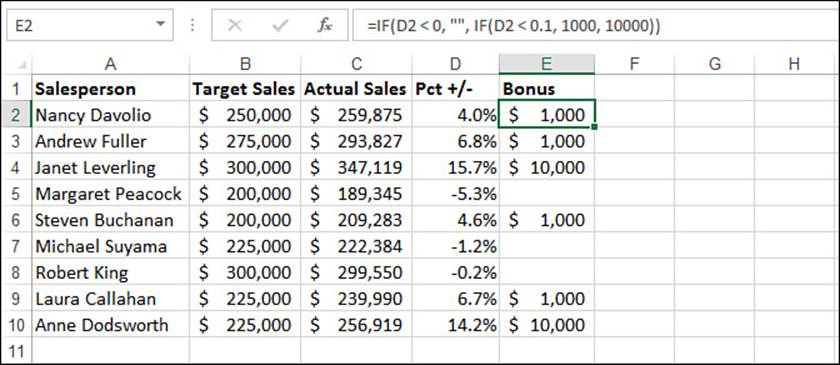
Figure 8.3 This worksheet uses nested IF() functions to calculate a tiered bonus payment.
The AND() Function
It’s often necessary to perform an action if and only if two conditions are true. For example, you might want to pay a salesperson a bonus if and only if dollar sales exceeded the budget and unit sales also exceeded the budget. If either the dollar sales or the unit sales fell below budget (or if they both fell below budget), no bonus is paid. In Boolean logic, this is called an And condition because one expression and another must be true for a positive result.
In Excel, And conditions are handled, appropriately enough, by the AND() logical function:
AND(logical1 [,logical2,...])

You can enter up to 255 logical conditions.
The AND() result is calculated as follows:
![]() If all the arguments return TRUE (or any nonzero number), AND() returns TRUE.
If all the arguments return TRUE (or any nonzero number), AND() returns TRUE.
![]() If one or more of the arguments return FALSE (or 0), AND() returns FALSE.
If one or more of the arguments return FALSE (or 0), AND() returns FALSE.
You can use the AND() function anywhere you would use a logical formula, but it’s most often pressed into service as the logical condition in an IF() function. In other words, if all the logical conditions in the AND() function are TRUE, IF() returns its value_if_true result; if one or more of the logical conditions in the AND() function are FALSE, IF() returns its value_if_false result.
For example, suppose you want to pay out a bonus only if a salesperson exceeds his budget for both dollar sales and unit sales. Assuming that the difference between the actual and budgeted dollar amounts is in cell B2 and the difference between the actual and budgeted unit amounts is in cell C2, here’s an example of a formula that determines whether a bonus is paid:
=IF(AND(B2 > 0, C2 > 0), "1000", "No bonus")
If the value in B2 is greater than 0 and the value in C2 is greater than 0, the formula returns 1000; otherwise, it returns No bonus.
Slotting Values into Categories
A good use for the AND() function is to slot items into categories that consist of a range of values. For example, suppose you have a set of poll or survey results, and you want to categorize these results based on the following age ranges: 18-34, 35-49, 50-64, and 65+. Assuming that each respondent’s age is in cell B9, the following AND() function can serve as the logical test for entry into the 18-34 category:
AND(B9 >= 18, B9 <= 34)
If the response is in C9, the following formula will display it if the respondent is in the 18-34 age group:
=IF(AND(B9 >= 18, B9 <= 34), C9, "")
Figure 8.4 tries this on some data. Here are the formulas used for the other age groups:
35-49: =IF(AND(B9 >= 35, B9 <= 49), C9, "")
50-64: =IF(AND(B9 >= 50, B9 <= 64), C9, "")
65+: =IF(B9 >= 65, C9, "")
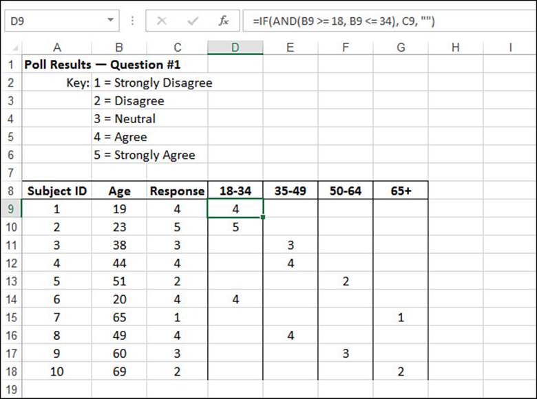
Figure 8.4 This worksheet uses the AND() function as the logical condition for an IF() function to slot poll results into age groups.
The OR() Function
Similar to an And condition is the situation when you need to take an action if one thing or another is true. For example, you might want to pay a salesperson a bonus if she exceeded the dollar sales budget or if she exceeded the unit sales budget. In Boolean logic, this is called an Orcondition.
You won’t be surprised to hear that Or conditions are handled in Excel by the OR() function:
OR(logical1 [,logical2,...])
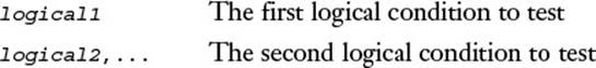
You can enter up to 255 logical conditions.
The OR() result is calculated as follows:
![]() If one or more of the arguments return TRUE (or any nonzero number), OR() returns TRUE.
If one or more of the arguments return TRUE (or any nonzero number), OR() returns TRUE.
![]() If all of the arguments return FALSE (or 0), OR() returns FALSE.
If all of the arguments return FALSE (or 0), OR() returns FALSE.
As with AND(), you use OR() wherever a logical expression is called for, most often within an IF() function. This means that if one or more of the logical conditions in the OR() function are TRUE, IF() returns its value_if_true result; if all the logical conditions in the OR()function are FALSE, IF() returns its value_if_false result.
For example, suppose you want to pay out a bonus only if a salesperson exceeds her budget for either dollar sales or unit sales (or both). Assuming that the difference between the actual and budgeted dollar amounts is in cell B2 and the difference between the actual and budgeted unit amounts is in cell C2, here’s an example of a formula that determines whether a bonus is paid:
=IF(OR(B2 > 0, C2 > 0), "1000", "No bonus")
If the value in B2 is greater than 0 or the value in C2 is greater than 0, the formula returns 1000; otherwise, it returns No bonus.
Note
The OR() function returns TRUE when one or more of its arguments are TRUE. However, in some cases, you want an expression to return TRUE only when just one of the arguments is TRUE. In that case, use the XOR() function, which returns TRUE when one and only one of its arguments evaluates to TRUE.
Applying Conditional Formatting with Formulas
In Chapter 1, “Getting the Most Out of Ranges,” you learned about the powerful conditional formatting features available in Excel. These features enable you to highlight cells, create top and bottom rules, and apply three types of formatting: data bars, color scales, and icon sets.
![]() For the details on conditional formatting, see “Applying Conditional Formatting to a Range,” p. 25.
For the details on conditional formatting, see “Applying Conditional Formatting to a Range,” p. 25.
Excel comes with another conditional formatting component that makes this feature even more powerful: You can apply conditional formatting based on the results of a formula. In particular, you can set up a logical formula as the conditional formatting criteria. If that formula returns TRUE, Excel applies the formatting to the cells; if the formula returns FALSE, instead, Excel doesn’t apply the formatting. In most cases, you use an IF() function, often combined with another logical function such as AND() or OR().
Before we get to an example, here are the basic steps to follow to set up formula-based conditional formatting:
1. Select the cells to which you want the conditional formatting applied.
2. Select Home, Conditional Formatting, New Rule. Excel displays the New Formatting Rule dialog box.
3. Click Use a Formula to Determine Which Cells to Format.
4. In the Format Values Where This Formula Is True range box, type your logical formula.
5. Click Format to open the Format Cells dialog box.
6. Use the Number, Font, Border, and Fill tabs to specify the formatting you want to apply and then click OK.
7. Click OK.
For example, suppose you have a range or table of items and you want to highlight those items that have the maximum and minimum values in a particular column. You could set up separate top and bottom rules, but you can make things easier and more flexible by instead using a logical formula.
How you go about this in a conditional formatting rule is a bit tricky, but it can be extremely powerful when you know the trick. First, you can use the MAX() worksheet function to determine the maximum value in a range. For example, if the range is D2:D10, then the following function returns the maximum:
MAX($D$2:$D$10)
However, a conditional formatting formula works only if it returns TRUE or FALSE, so you need to create a comparison formula:
=MAX($D$2:$D$10)=$D2
There are two things to note here: First, you compare the range to the first value in the range; second, the cell address uses the mixed-reference format $D2, which tells Excel to keep the column (D) fixed, while varying the row number.
Next, you can use the MIN() function to determine the minimum, so you create a similar comparison formula:
=MIN($D$2:$D$10)=$D2
Finally, you want to check each cell in the column to see if it’s the maximum or the minimum, so you need to combine these expressions by using the OR() function, like so:
=OR(MAX($D$2:$D$10)=$D2, MIN($D$2:$D$10)=$D2)
Figure 8.5 shows a range of sales results (A2:E10) that are conditionally formatted using the preceding formula. This shows which reps had the maximum and minimum percentage differences between target sales and actual sales (column D).
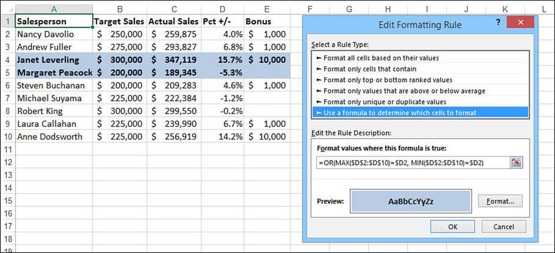
Figure 8.5 A range of sales rep data conditionally formatted using a logical formula.
Combining Logical Functions with Arrays
When you combine the array formulas you learned about in Chapter 4, “Creating Advanced Formulas,” with IF(), you can perform some remarkably sophisticated operations. Arrays enable you to do things such as apply the IF() logical condition across a range as well as sum only those cells in a range that meet the IF() condition.
![]() To learn about array formulas, see “Working with Arrays,” p. 87.
To learn about array formulas, see “Working with Arrays,” p. 87.
Applying a Condition Across a Range
Using AND() as the logical condition in an IF() function is useful for perhaps three or four expressions. After that, it just gets too unwieldy to enter all those logical expressions. If you’re essentially running the same logical test on a number of different cells, a better solution is to applyAND() to a range and enter the formula as an array.
For example, suppose that you want to sum the cells in the range B3:B7 but only if all those cells contain values greater than 0. Here’s an array formula to do this:
{=IF(AND(B3:B7 > 0), SUM(B3:B7), "")}
Note
Recall from Chapter 4 that you don’t include the braces ({ }) when you enter an array formula. Type the formula without the braces and then press Ctrl+Shift+Enter.
This is useful in a worksheet in which you might not have all the numbers yet, and you don’t want a total entered until the data is complete. Figure 8.6 shows an example. The array formula in B8 is the same as the previous one. The array formula in B16 returns nothing because cell B14 is blank.
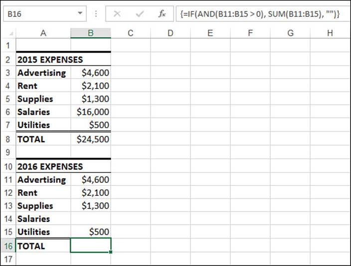
Figure 8.6 This worksheet uses IF(), AND(), and SUM() in two array formulas (B8 and B16) to total a range only if all the cells have nonzero values.
Operating Only on Cells That Meet a Condition
In the previous section, you saw how to use an array formula to perform an action only if a certain condition is met across a range of cells. A related scenario arises when you want to perform an action on a range, but only on cells that meet a certain condition. For example, you might want to sum only values that are positive.
To do this, you need to move the operation outside the IF() function. For example, here’s an array formula that sums only values in the range B3:B7 that contain positive values:
{=SUM(IF(B3:B7 > 0, B3:B7, 0))}
The IF() function returns an array of values based on the condition (the cell value if it’s positive; 0 otherwise), and the SUM() function adds those returned values.
For example, suppose you have a series of investments that mature in various years. It would be nice to set up a table that lists these years and tells you the total value of the investments that mature in each year. Figure 8.7 shows a worksheet set up to do just that.
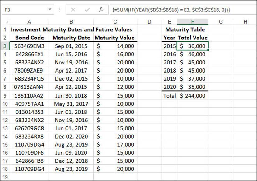
Figure 8.7 This worksheet uses array formulas to sum the yearly maturity values of various investments.
The investment maturity dates are in column B, the investment values at maturity are shown in column C, and the various maturity years are in column E. To calculate the maturity total for 2015, for example, the following array formula is used:
{=SUM(IF(YEAR($B$3:$B$18) = E3, $C$3:$C$18, 0))}
The IF() function compares the year value in cell E3 (2015) with the year component of the maturity dates in range B3:B18. For cells in which these are equal, IF() returns the corresponding value in column C; otherwise, it returns 0. The SUM() function then adds these returned values.
Note
In Figure 8.7, notice that, with the exception of the reference to cell E3, I used absolute references so the formula can be filled down to the other years.
Determining Whether a Value Appears in a List
Many spreadsheet applications require you to look up a value in a list. For example, you might have a table of customer discounts in which the percentage discount is based on the number of units ordered. For each customer order, you need to look up the appropriate discount, based on the total units in the order. Similarly, a teacher might convert a raw test score into a letter grade by referring to a table of conversions.
You’ll see some sophisticated tools for looking up values in Chapter 9, “Working with Lookup Functions.” However, array formulas combined with logical functions also offer some tricks for looking up values.
For example, suppose that you want to know whether a certain value exists in an array. You can use the following general formula, entered into a single cell as an array:
{=OR(value = range)}
Here, value is the value you want to search for, and range is the range of cells in which to search. For example, Figure 8.8 shows a list of customers with overdue accounts. You enter the account number of the customer in cell B1, and cell B2 tells you whether the number appears in the list.
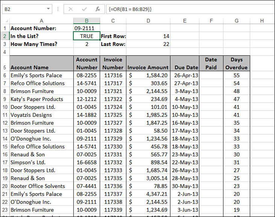
Figure 8.8 This worksheet uses the OR() function in an array formula to determine whether a value appears in a list.
Here’s the array formula in cell B2:
{=OR(B1 = B6:B29)}
The array formula checks each value in the range B6:B29 to see whether it equals the value in cell B1. If any one of those comparisons is true, OR() returns TRUE, which means the value is in the list.
Tip
As a similar example, here’s an array formula that returns TRUE if a particular account number is not in the list:
{=AND(B1 <> B6:B29)}
The formula checks each value in B6:B29 to see whether it does not equal the value in B1. If all those comparisons are true, AND() returns TRUE, which means the value is not in the list.
Counting Occurrences in a Range
Now you know how to find out whether a value appears in a list, but what if you need to know how many times the value appears? The following formula does the job:
{=SUM(IF(value = range, 1, 0))}
Again, value is the value you want to look up, and range is the range for searching. In this array formula, the IF() function compares value with every cell in range. The values that match return 1, and those that don’t return 0. The SUM() function adds these returned values, and the final total is the number of occurrences of value. Here’s a formula that does this for our list of overdue invoices:
{=SUM(IF(B1 = B6:B29, 1, 0))}
Figure 8.9 shows this formula in action (see cell B3).
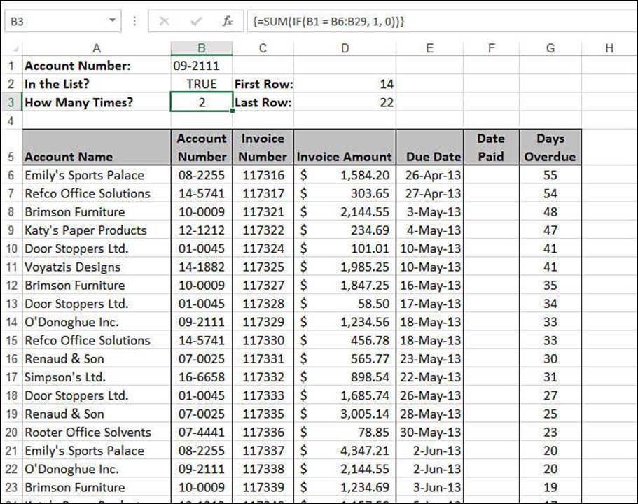
Figure 8.9 This worksheet uses SUM() and IF() in an array formula to count the number of occurrences of a value in a list.
Note
The generic array formula {=SUM(IF(condition, 1, 0))} is useful in any context where you need to count the number of occurrences in which condition returns TRUE. The condition argument is normally a logical formula that compares a single value with each cell in a range of values. However, it’s also possible to compare two ranges, as long as they’re the same shape (that is, they have the same number of rows and columns). For example, suppose that you want to compare the values in two ranges named Range1 and Range2 to see if any of the values are different. Here’s an array formula that does this:
{=SUM(IF(Range1 <> Range2, 1, 0))}
This formula compares the first cell in Range1 with the first cell in Range2, the second cell in Range1 with the second cell in Range2, and so on. Each time the values don’t match, the comparison returns 1; otherwise, it returns 0. The sum of these comparisons is the number of different values between the two ranges.
Determining Where a Value Appears in a List
What if you want to know not just whether a value appears in a list but where it appears in the list? You can do this by getting the IF() function to return the row number for a positive result:
IF(value = range, ROW(range), "")
Whenever value equals one of the cells in range, the IF() function uses ROW() to return the row number; otherwise, it returns the empty string.
To return that row number, use either the MIN() function or the MAX() function, which returns the minimum or maximum, respectively, in a collection of values. The trick here is that both functions ignore null values, so applying this to the array that results from the previous IF()expression tells where the matching values are:
![]() To get the first instance of the value, use the MIN() function in an array formula, like so:
To get the first instance of the value, use the MIN() function in an array formula, like so:
{=MIN(IF(value = range, ROW(range), ""))}
![]() To get the last instance of the value, use the MAX() function in an array formula, as shown here:
To get the last instance of the value, use the MAX() function in an array formula, as shown here:
{=MAX(IF(value = range, ROW(range), ""))}
Here are the formulas you would use to find the first and last occurrences in the previous list of overdue invoices:
{=MIN(IF(B1 = B6:B29, ROW(B6:B29), ""))}
{=MAX(IF(B1 = B6:B29, ROW(B6:B29), ""))}
Figure 8.10 shows the results (with the row of the first occurrence in cell D2 and the row of the last occurrence in cell D3).
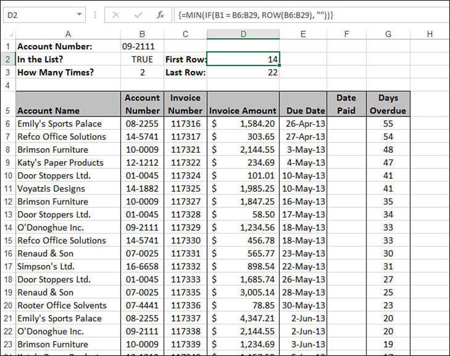
Figure 8.10 This worksheet uses MIN(), MAX(), ROW(), and IF() in array formulas to return the row numbers of the first (cell D2) and last (cell D3) occurrences of a value in a list.
Tip
It’s also possible to determine the address of the cell that contains the first or last occurrence of a value in a list. To do this, use the ADDRESS() function, which returns an absolute address, given a row and column number:
{=ADDRESS(MIN(IF(B1 = B6:B29, ROW(B6:B29), "")), COLUMN(B6:B29))}
{=ADDRESS(MAX(IF(B1 = B6:B29, ROW(B6:B29), "")), COLUMN(B6:B29))}
Case Study: Building an Accounts Receivable Aging Worksheet
If you use Excel to store accounts receivable data, it’s a good idea to set up an aging worksheet that shows past-due invoices, calculates the number of days past due, and groups the invoices into past-due categories (1-30 days, 31-60 days, and so on).
Figure 8.11 shows a simple implementation of an accounts receivable database. For each invoice, the due date (column D) is calculated by adding 30 to the invoice date (column C). Column E subtracts the due date (column D) from the current date (in cell B1) to calculate the number of days each invoice is past due.
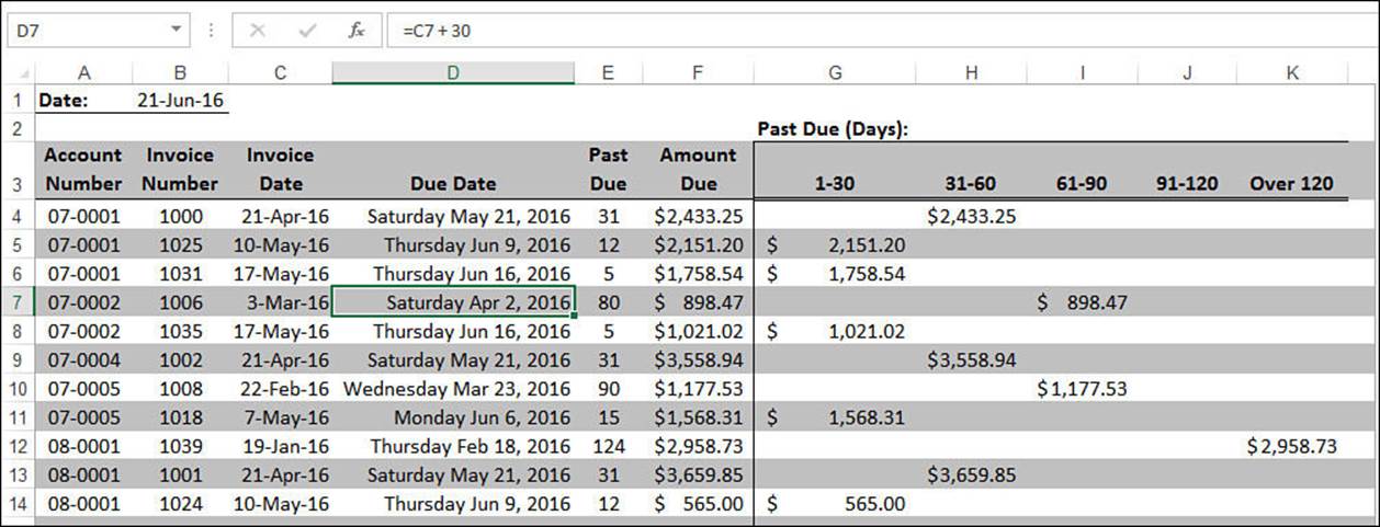
Figure 8.11 A simple accounts receivable database.
Calculating a Smarter Due Date
You might have noticed a problem with the due dates in Figure 8.11: Several of the dates, including the date in cell D7, fall on weekends. The problem here is that the due date calculation just adds 30 to the invoice date. To avoid weekend due dates, you need to test whether the invoice date plus 30 falls on a Saturday or Sunday. The WEEKDAY() function helps because it returns 7 if the date is a Saturday, and 1 if the date is a Sunday.
So, to check for a Saturday, you could use the following formula:
=IF(WEEKDAY(C4 + 30) = 7, C4 + 32, C4 + 30)
Here, I’m assuming that the invoice date resides in cell C4. If WEEKDAY(C4 + 30) returns 7, the date is a Saturday, so you add 32 to C4 instead (to make the due date the following Monday). Otherwise, you just add 30 days as usual.
Checking for a Sunday is similar:
=IF(WEEKDAY(C4 + 30) = 1, C4 + 31, C4 + 30)
The problem, though, is that you need to combine these two tests into a single formula. To do that, you can nest one IF() function inside another. Here’s how it works:
=IF(WEEKDAY(C4+30) = 7, C4+32, IF(WEEKDAY(C4+30) = 1, C4+31, C4+30))
The main IF() checks whether the date is a Saturday. If it is, you add 32 days to C4; otherwise, the formula runs the second IF(), which checks for Sunday. Figure 8.12 shows the revised aging sheet with the nonweekend due dates in column D.
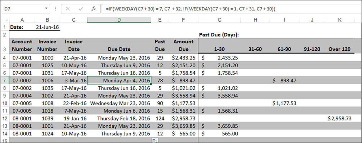
Figure 8.12 The revised worksheet uses the IF() and WEEKDAY() functions to ensure that due dates don’t fall on weekends.
![]() For calculating due dates based on workdays (that is, excluding weekends and holidays), Excel has a function named WORKDAY() that handles this calculation with ease; see “A Workday Alternative: The WORKDAY() Function,” p. 216.
For calculating due dates based on workdays (that is, excluding weekends and holidays), Excel has a function named WORKDAY() that handles this calculation with ease; see “A Workday Alternative: The WORKDAY() Function,” p. 216.
Aging Overdue Invoices
For cash-flow purposes, you also need to correlate the invoice amounts with the number of days past due. Ideally, you’d like to see a list of invoice amounts that are between 1 and 30 days past due, between 31 and 60 days past due, and so on. Figure 8.13 shows one way to set up accounts receivable aging.
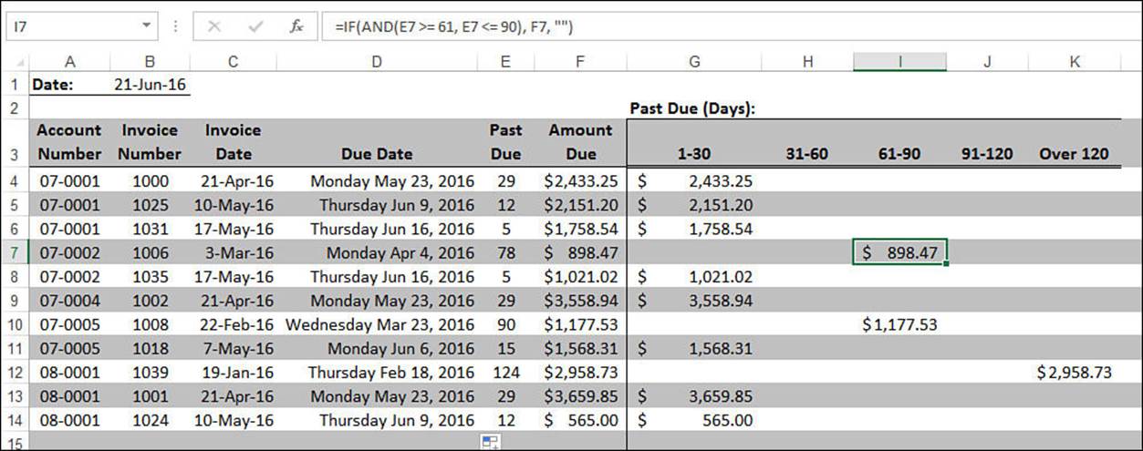
Figure 8.13 Using IF() and AND() to categorize past-due invoices for aging purposes.
![]() The worksheet in Figures 8.11 through 8.13 uses ledger shading for easier reading. To learn how to apply ledger shading automatically, see “Creating Ledger Shading,” p. 251.
The worksheet in Figures 8.11 through 8.13 uses ledger shading for easier reading. To learn how to apply ledger shading automatically, see “Creating Ledger Shading,” p. 251.
The aging worksheet calculates the number of days past due by subtracting the due date from the date shown in cell B1. If you calculate days past due using only workdays (weekends and holidays excluded), a better choice is the NETWORKDAYS() function, covered in Chapter 10, “Working with Date and Time Functions.”
![]() To learn more about the NETWORKDAYS() function, see “NETWORKDAYS(): Calculating the Number of Workdays Between Two Dates,” p. 225.
To learn more about the NETWORKDAYS() function, see “NETWORKDAYS(): Calculating the Number of Workdays Between Two Dates,” p. 225.
For the invoice amounts shown in column G (1-30 days), the sheet uses the following formula (which appears in G4):
=IF(E4 <= 30, F4, "")
If the number of days the invoice is past due (cell E4) is less than or equal to 30, the formula displays the amount (from cell F4); otherwise, it displays a blank.
The amounts in column H (31-60 days) are a little trickier. Here, you need to check whether the number of days past due is greater than or equal to 31 days and less than or equal to 60 days. To accomplish this, you can press the AND() function into service:
=IF(AND(E4 >= 31, E4 <= 60), F4, "")
The AND() function checks two logical expressions: E4> = 31 and E4 <= 60. If both are true, AND() returns TRUE, and the IF() function displays the invoice amount. If one of the logical expressions isn’t true (or if they’re both not true), AND() returns FALSE, and the IF()function displays a blank. Similar formulas appear in column I (61-90 days) and column J (91-120 days). Column K (Over 120) looks for past-due values that are greater than 120.
Getting Data with Information Functions
Excel’s information functions return data concerning cells, worksheets, and formula results. Table 8.2 lists all the information functions.
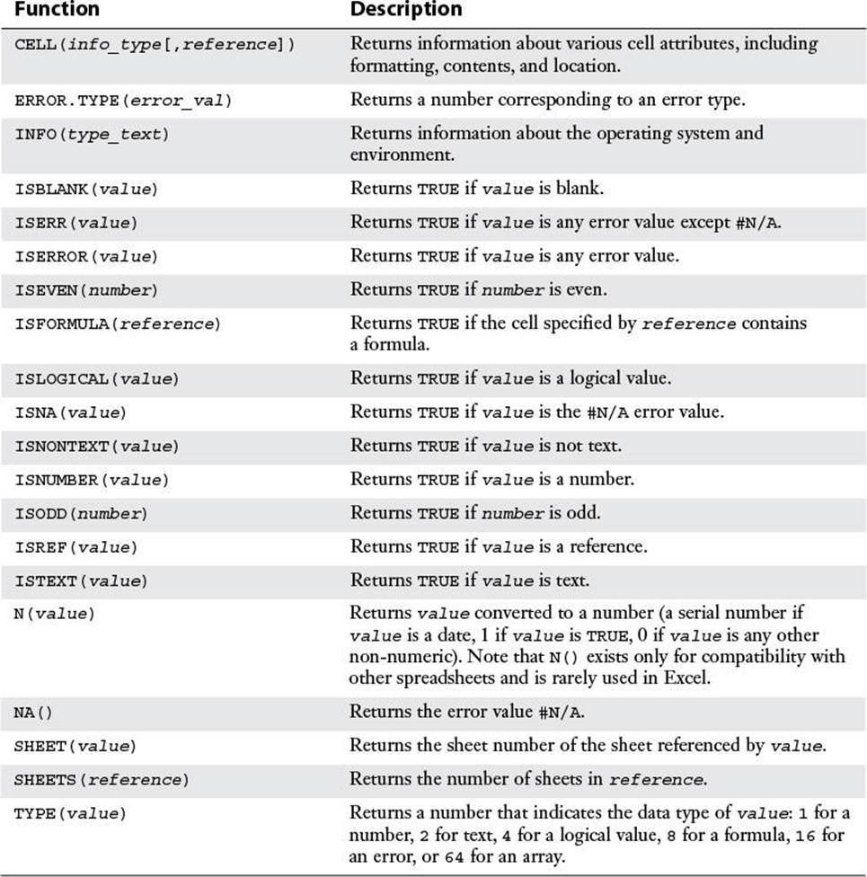
Table 8.2 Excel’s Information Functions
The rest of this chapter takes you through the details of several of these functions.
The CELL() Function
CELL() is one of the most useful information functions. Its job is to return information about a particular cell:
CELL(info_type, [reference])
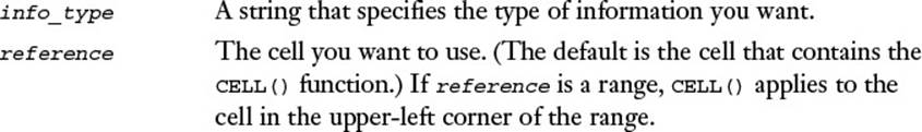
Table 8.3 lists the various possibilities for the info_type argument.
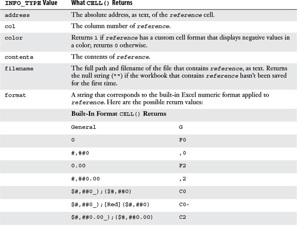
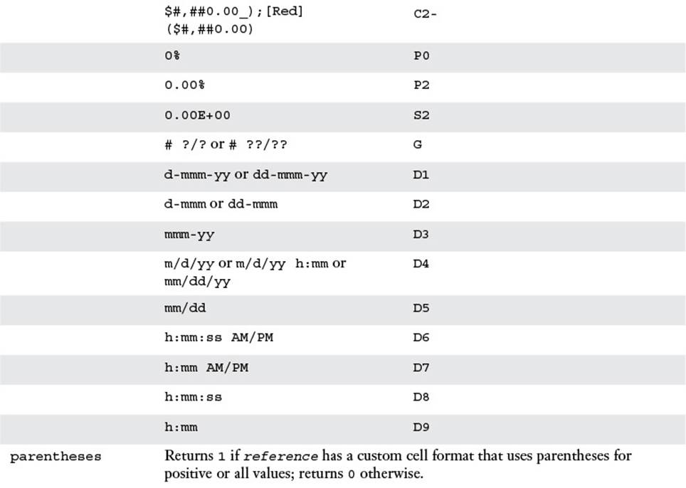
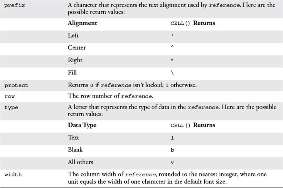
Table 8.3 The CELL() Function’s info_type Argument
Figure 8.14 shows how the CELL() function works.
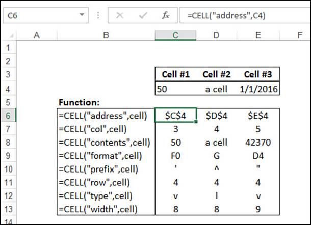
Figure 8.14 Some examples of the CELL() function.
The ERROR.TYPE() Function
The ERROR.TYPE() function returns a value that corresponds to a specific Excel error value:
ERROR.TYPE(error_val)
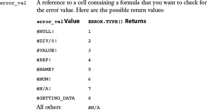
You most often use the ERROR.TYPE() function to intercept an error and then display a more useful or friendly message. You do this by using the IF() function to see if ERROR.TYPE() returns a value less than or equal to 7; if so, the cell in question contains an error value. Because theERROR.TYPE() returns value ranges from 1 to 8, you can apply the return value to the CHOOSE() function to display the error message.
![]() For the details of the CHOOSE() function, see “The CHOOSE() Function,” p. 193.
For the details of the CHOOSE() function, see “The CHOOSE() Function,” p. 193.
Here’s a formula that does all that. (I’ve split the formula so that different parts appear on different lines to make it easier for you to see what’s going on.)
=IF(ERROR.TYPE(D8) <= 8, ***ERROR IN " & CELL("address",D8) & ": " & CHOOSE(ERROR.TYPE(D8),"The ranges do not intersect", "The divisor is 0", "Wrong data type in function argument", "Invalid cell reference", "Unrecognized range or function name", "Number error in formula", "Inappropriate function argument" "Waiting for query data"))
Figure 8.15 shows this formula in an example. (Note that the formula displays #N/A when there is no error; this is the return value of ERROR.TYPE() when there is no error.)
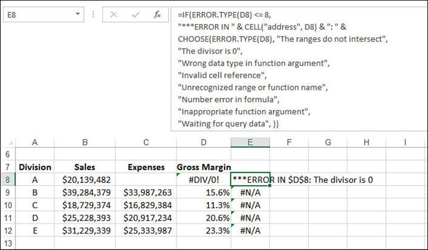
Figure 8.15 A formula that uses IF() and ERROR_TYPE() to return a more descriptive error message to the user.
The INFO() Function
The INFO() function is seldom used, but it’s handy when you do need it because it gives you information about the current operating environment:
INFO(type_text)
![]()
Table 8.4 lists the possible values for the type_text argument.
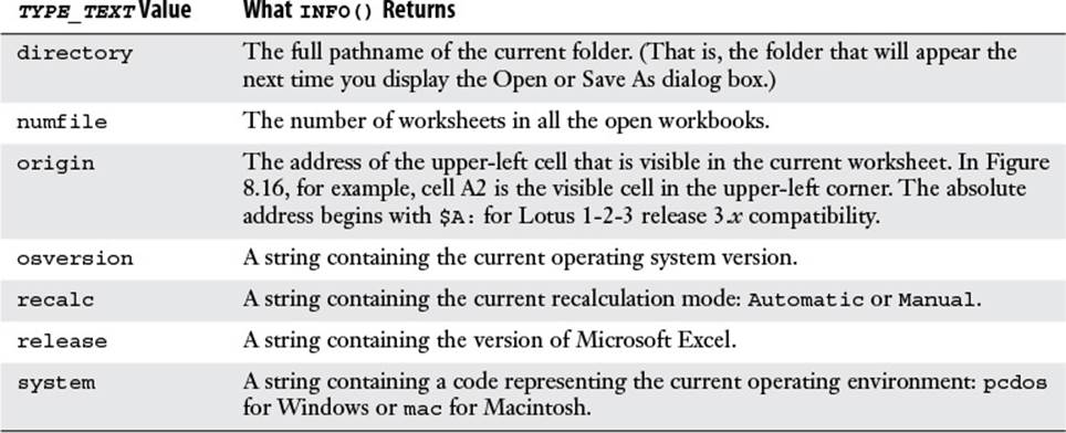
Table 8.4 The INFO() Function’s type_text Argument
Figure 8.16 shows the INFO() function at work.
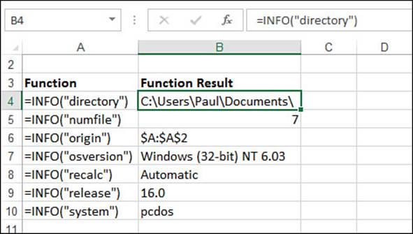
Figure 8.16 The INFO() function in action.
The SHEET() and SHEETS() Functions
Excel includes two information functions—SHEET() and SHEETS()—that return information about the worksheets in a workbook. You use the SHEET() function to return a sheet number using the following syntax:
SHEET([value])
![]()
For example, the formula =SHEET() returns the number of the sheet that contains the formula, where 1 is the first sheet in the workbook, 2 is the second sheet, and so on. Note that Excel counts all sheet types, including worksheets and chart sheets.
If a worksheet has the name Budget, then the formula =SHEET("Budget") returns its sheet number. Alternatively, you can use a cell reference within that sheet, such as SHEET(Budget!A1).
You use the SHEETS() function (which takes no arguments) to return the total number of worksheets in the current workbook.
The IS Functions
Excel’s so-called IS functions are Boolean functions that return either TRUE or FALSE, depending on the argument they’re evaluating:
ISBLANK(value)
ISERR(value)
ISERROR(value)
ISEVEN(number)
ISFORMULA(reference)
ISLOGICAL(value)
ISNA(value)
ISNONTEXT(value)
ISNUMBER(value)
ISODD(number)
ISREF(value)
ISTEXT(value)
The operation of these functions is straightforward, so rather than run through the specifics of all 11 functions, the next few sections show you some interesting and useful techniques that make use of these functions.
Counting the Number of Blanks in a Range
When putting together the data for a worksheet model, it’s common to pull the data from various sources. Unfortunately, this often means that the data arrives at different times, and you end up with an incomplete model. If you’re working with a big list, you might want to keep a running total of the number of pieces of data you’re still missing.
This is the perfect opportunity to break out the ISBLANK() function and plug it into the array formula for counting that you learned earlier:
{=SUM(IF(ISBLANK(range), 1, 0))}
The IF() function runs through the range, looking for blank cells. Each time it comes across a blank cell, it returns 1; otherwise, it returns 0. The SUM() function adds the results to give the total number of blank cells. Figure 8.17 shows an example (see cell G1).
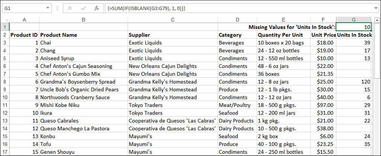
Figure 8.17 As shown in cell G1, you can plug ISBLANK() into the array counting formula to count the number of blank cells in a range.
Tip
Using an array formula to count blank cells is fine, but it’s not the easiest way to go about it. In most cases, you’re better off just using the COUNTBLANK(range) function, which counts the number of blank cells that occur in the range specified by the range argument.
Checking a Range for Non-Numeric Values
A similar idea is to check a range on which you’ll be performing a mathematical operation to see if it holds any cells that contain non-numeric values. In this case, you plug the ISNUMBER() function into the array counting formula and then return 0 for each TRUE result and 1 for eachFALSE result. Here’s the general formula:
{=SUM(IF(ISNUMBER(range), 0, 1))}
Counting the Number of Errors in a Range
For the final counting example, it’s often nice to know not only whether a range contains an error value but also how many such values it contains. This is easily done using the ISERROR() function and the array counting formula:
{=SUM(IF(ISERROR(range), 1, 0))}
Ignoring Errors When Working with a Range
Sometimes, you have to work with ranges that contain error values. For example, suppose that you have a column of gross margin results (which require division), but one or more of the cells are showing the #DIV/0! error because you’re missing data. You could wait until the missing data is added to the model, but it’s often necessary to perform preliminary calculations. For example, you might want to take the average of the results that you do have.
To do this efficiently, you need some way of bypassing the error values. Again, this is possible by using the ISERROR() function plugged into an array formula. For example, here’s a general formula for taking an average across a range while ignoring any error values:
{=AVERAGE(IF(ISERROR(range), "", range))}
Figure 8.18 provides an example.
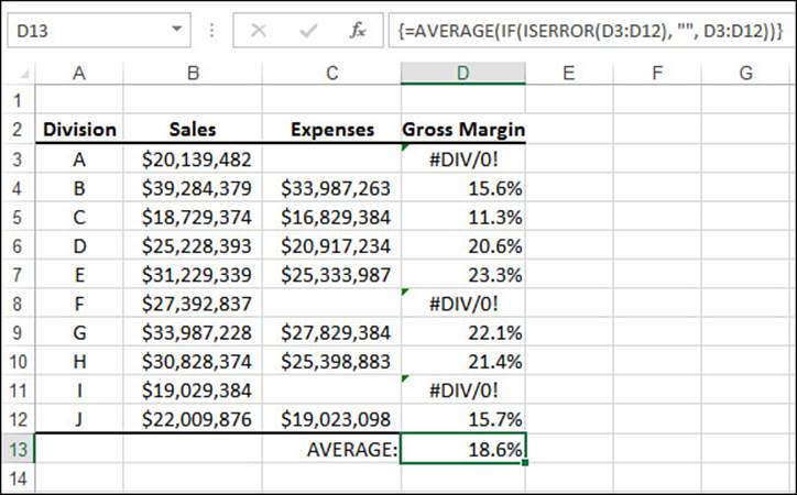
Figure 8.18 As shown in cell D13, you can use ISERROR() in an array formula to run an operation on a range while ignoring any errors in the range.
From Here
![]() For the details on conditional formatting, see “Applying Conditional Formatting to a Range,” p. 25.
For the details on conditional formatting, see “Applying Conditional Formatting to a Range,” p. 25.
![]() To learn about array formulas, see “Working with Arrays,” p. 87.
To learn about array formulas, see “Working with Arrays,” p. 87.
![]() To learn about the #DIV/0! error, see “#DIV/0!,” p. 112.
To learn about the #DIV/0! error, see “#DIV/0!,” p. 112.
![]() To learn about the IFERROR() and IFNA() functions, see “Handling Formula Errors with IFERROR(),” p. 118.
To learn about the IFERROR() and IFNA() functions, see “Handling Formula Errors with IFERROR(),” p. 118.
![]() For a general discussion of function syntax, see “The Structure of a Function,” p. 130.
For a general discussion of function syntax, see “The Structure of a Function,” p. 130.
![]() For the details on the REPT() function, see “The REPT() Function: Repeating a Character or String,” p. 150.
For the details on the REPT() function, see “The REPT() Function: Repeating a Character or String,” p. 150.
![]() To learn about extracting a name from a string, see “Extracting a First Name or Last Name,” p. 156.
To learn about extracting a name from a string, see “Extracting a First Name or Last Name,” p. 156.
![]() For the details of the CHOOSE() function, see “The CHOOSE() Function,” p. 193.
For the details of the CHOOSE() function, see “The CHOOSE() Function,” p. 193.
![]() To learn how to use the WORKDAY() function, see “A Workday Alternative: The WORKDAY() Function,” p. 216.
To learn how to use the WORKDAY() function, see “A Workday Alternative: The WORKDAY() Function,” p. 216.
![]() To learn how to apply ledger shading automatically, see “Creating Ledger Shading,” p. 251.
To learn how to apply ledger shading automatically, see “Creating Ledger Shading,” p. 251.
![]() For information on referencing tables in formulas, see “Referencing Tables in Formulas,” p. 309.
For information on referencing tables in formulas, see “Referencing Tables in Formulas,” p. 309.
All materials on the site are licensed Creative Commons Attribution-Sharealike 3.0 Unported CC BY-SA 3.0 & GNU Free Documentation License (GFDL)
If you are the copyright holder of any material contained on our site and intend to remove it, please contact our site administrator for approval.
© 2016-2026 All site design rights belong to S.Y.A.