Excel 2016 Formulas (2016)
PART V
Miscellaneous Formula Techniques
· Chapter 16: Importing and Cleaning Data
· Chapter 17: Charting Techniques
· Chapter 18: Pivot Tables
· Chapter 19: Conditional Formatting
· Chapter 20: Using Data Validation
· Chapter 21: Creating Megaformulas
· Chapter 22: Tools and Methods for Debugging Formulas
Chapter 16
Importing and Cleaning Data
In This Chapter
· Ways to import data into Excel
· Many techniques to manipulate and clean data
· Using the new Fill Flash feature
· A checklist for data cleaning
· Exporting data to other formats
One common use for Excel is as a tool to “clean up” data. Cleaning up data involves getting raw data into a worksheet and then manipulating it so it conforms to various requirements. In the process, the data will be made consistent so that it can be properly analyzed.
This chapter describes various ways to get data into a worksheet and provides some tips to help you clean it up.
A Few Words About Data
Data is everywhere. For example, if you run a website, you’re collecting data continually, and you may not even know it. Every visit to your site generates information stored in a file on your server. This file contains lots of useful information—if you take the time to examine it.
That’s just one example of data collection. Virtually every automated system collects data and stores it. Most of the time, the system that collects the data is also equipped to verify and analyze it. Not always, though. And, of course, data is also collected manually. An example is a telephone survey.
Excel is a good tool for analyzing data, and it’s often used to summarize the information and display it in the form of tables and charts. But often, the data that’s collected isn’t perfect. For one reason or another, it needs to be cleaned up before it can be analyzed.
Importing Data
Before you can do anything with data, you must get it into a worksheet. Excel can import most common text file formats and can retrieve data from websites.
Importing from a file
This section describes file types that Excel can open directly, using the File ➜ Open command. Figure 16.1 shows the list of file filter options you can specify from this dialog box.

Figure 16.1 Filtering by file extension in the Open dialog box.
Spreadsheet file formats
In addition to the current file formats (XLSX, XLSM, XLSB, XLTX, XLTM, and XLAM), Excel 2016 can open workbook files from all previous versions of Excel:
§ XLS: Binary files created by Excel 4, Excel 95, Excel 97, Excel 2000, Excel 2002, and Excel 2003
§ XLM: Binary files that contain Excel 4 macros (no data)
§ XLT: Binary files for an Excel template
§ XLA: Binary files for an Excel add-in
Excel can also open one file format created by other spreadsheet products:
§ ODS: OpenDocument spreadsheet. These files are produced by a variety of open-source software, including Google Drive, OpenOffice, LibreOffice, StarOffice, and several others.
Note that Excel does not support Lotus 1-2-3 files, Quattro Pro files, or Microsoft Works files.
Database file formats
Excel 2016 can open the following database file formats:
§ Access files: These files have various extensions, including MDB and ACCDB.
§ dBase files: These are produced by dBase III and dBase IV. Excel does not support dBase II files.
In addition, Excel supports various types of database connections that enable you to access data selectively. For example, you can perform a query on a large database to retrieve only the records you need (rather than the entire database).
Text file formats
A text file contains raw characters with no formatting. Excel can open most types of text files:
§ CSV: Comma-separated values. Columns are delimited with a comma, and rows are delimited with a carriage return.
§ TXT: Columns are delimited with a tab, and rows are delimited with a carriage return.
§ PRN: Columns are delimited with multiple space characters, and rows are delimited with a carriage return. Excel imports this type of file into a single column.
§ DIF: The file format originally used by the VisiCalc spreadsheet. Rarely used.
§ SYLK: The file format originally used by Multiplan. Rarely used.
Most of these text file types have variants. For example, text files produced by a Mac computer have different end-of-row characters. Excel can usually handle the variants without a problem.
When you attempt to open a text file in Excel, the Text Import Wizard might kick in to help you specify how you want the data to be retrieved.
![]() Tip
Tip
To bypass the Text Import Wizard, press Shift while you click the Open button in the Open dialog box.
![]() When Excel can’t open a file
When Excel can’t open a file
If Excel doesn’t support a particular file form, don’t be too quick to give up. Other folks have likely had the same problem. Try searching the web for the file extension, plus the word excel. Maybe a file converter is available, or someone has figured out how to use an intermediary program to open the file and export it into a format that Excel recognizes.
Importing HTML files
Excel can open most HTML files, which can be stored on your local drive or on a web server. Choose File ➜ Open and locate the HTML file. If the file is on a web server, copy the URL and paste it into the File Name field in the Open dialog box.
The way the HTML code renders in Excel varies considerably. Sometimes the HTML file may look exactly as it does in a browser. Other times, it may bear little resemblance, especially if the HTML file uses cascading style sheets (CSS) for layout.
![]() Cross-Ref
Cross-Ref
In some cases, you can access data on the Web by using a Web Query (Data ➜ Get External Data ➜ From Web).
Importing XML files
XML (eXtensible Markup Language) is a text file format suitable for structured data. Data is enclosed in tags, which also serve to describe the data.
Excel can open XML files, and simple files will display with little or no effort. Complex XML files will require some work, however. A discussion of this topic is beyond the scope of this book. You’ll find information about getting data from XML files in Excel’s Help system and online.
Importing a text file into a specified range
If you need to insert a text file into a specific range in a worksheet, you might think that your only choice is to import the text into a new workbook and then to copy the data and paste it to the range where you want it to appear. However, you can do it in a more direct way.
Figure 16.2 shows a small CSV file. The following instructions describe how to import this file, named monthly.csv, beginning at cell C3.
1. Choose Data ➜ Get External Data ➜ From Text to display the Import Text File dialog box.
2. Navigate to the folder that contains the text file.
3. Select the file from the list and then click the Import button to display the Text Import Wizard.
4. Use the Text Import Wizard to specify how the data will be imported. For a CSV file, specify Delimited with a Comma Delimiter.
5. Click the Finish button. Excel displays the Import Data dialog box, shown in Figure 16.3.
6. In the Import Data dialog box, click the Properties button to display the External Data Range Properties dialog box.
7. In the External Data Range Properties dialog box, deselect the Save Query Definition check box and click OK to return to the Import Data dialog box.
8. In the Import Data dialog box, specify the location for the imported data. (It can be a cell in an existing worksheet or a new worksheet.)
9. Click OK, and Excel imports the data (see Figure 16.4).
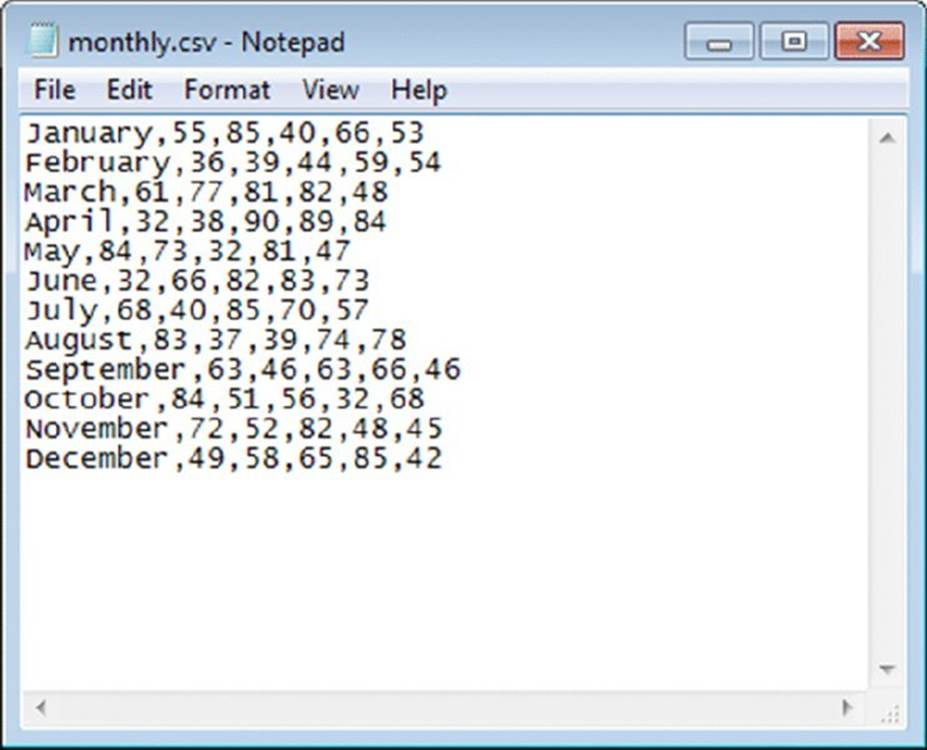
Figure 16.2 This CSV file will be imported into a range.
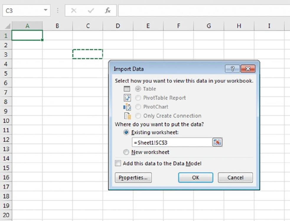
Figure 16.3 Using the Import Data dialog box to import a CSV file at a particular location.
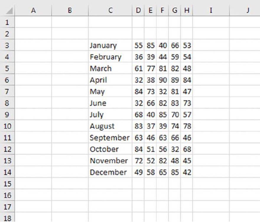
Figure 16.4 This range contains data imported directly from a CSV file.
![]() Note
Note
You can ignore Step 7 if the data you’re importing will be changing. By saving the query definition, you can quickly update the imported data by right-clicking any cell in the range and choosing Refresh Data.
Copying and pasting data
If all else fails, you can try standard copy and paste techniques. If you can copy data from an application (for example, a word processing program or a document displayed in a PDF viewer), chances are good that you can paste it into an Excel workbook. For best results, try pasting using the Home ➜ Clipboard ➜ Paste ➜ Paste Special command and employing the various paste options listed. Usually, pasted data requires some cleanup.
Data Cleanup Techniques
This section discusses a variety of techniques that you can use to clean up data in a worksheet.
![]() Cross-Ref
Cross-Ref
Chapter 5, “Manipulating Text,” contains additional examples of text-related formulas that may be helpful when cleaning data.
Removing duplicate rows
If data is compiled from multiple sources, it may contain duplicate rows. Most of the time, you want to eliminate the duplicates. In the past, removing duplicate data was essentially a manual task, although it could be automated by using a fairly nonintuitive advanced filter technique. Now removing duplicate rows is easy, thanks to Excel’s Remove Duplicates command (introduced in Excel 2007).
Start by moving the cell cursor to any cell within your data range. Choose Data ➜ Data Tools ➜ Remove Duplicates, and Excel displays the Remove Duplicates dialog box shown in Figure 16.5.
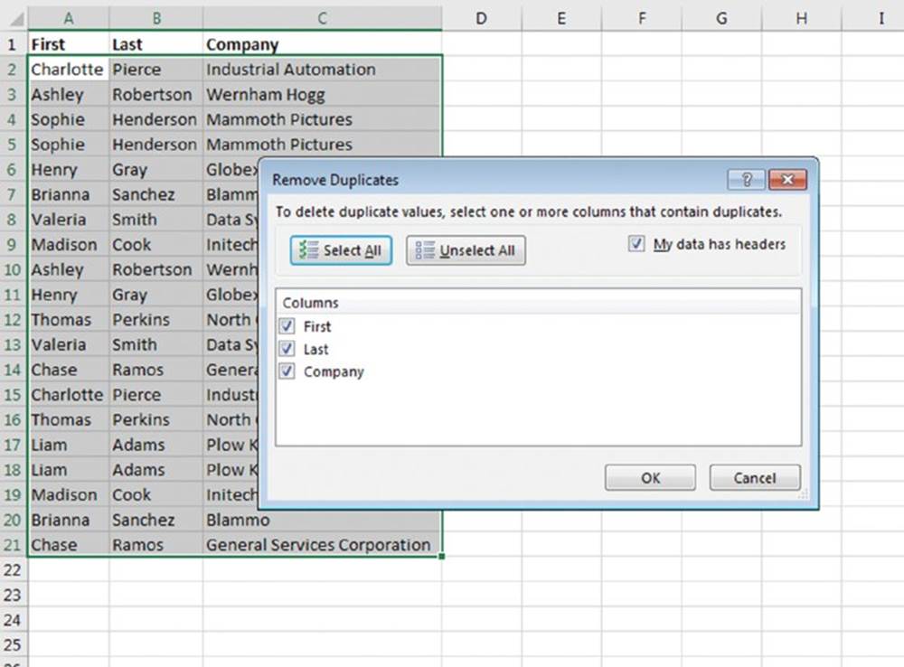
Figure 16.5 Use the Remove Duplicates dialog box to delete duplicate rows.
![]() Note
Note
If your data is in a table, you can also use Table Tools ➜ Design ➜ Data Tools ➜ Remove Duplicates. These two commands work the same.
The Remove Duplicates dialog box lists all the columns in your data range or table. Place a check mark next to the columns that you want to be included in the duplicate search. Most of the time, you’ll want to select all the columns, which is the default. Click OK, and Excel weeds out the duplicate rows and displays a message that tells you how many duplicates it removed. It would be nice if Excel gave you the option to just highlight the duplicates so you could look them over, but it doesn’t. If Excel deletes too many rows, you can undo the procedure by clicking Undo on the Quick Access Toolbar (or by pressing Ctrl+Z).
When you select all columns in the Remove Duplicates dialog box, Excel deletes a row only if the content of every column is duplicated. In some situations, you may not care about matching some columns, so you would deselect those columns in the Remove Duplicates dialog box. For example, if each row has a unique ID code, Excel would never find duplicate rows, so you’d want to uncheck that column in the Remove Duplicates dialog box.
When duplicate rows are found, the first row is kept, and subsequent duplicate rows are deleted.
![]() Warning
Warning
Duplicate values are determined by the value displayed in the cell—not necessarily the value stored in the cell. For example, assume that two cells contain the same date. One of the dates is formatted to display as 5/15/2013, and the other is formatted to display as May 15, 2013. When removing duplicates, Excel considers these dates to be different. Similarly, values that are formatted differently are considered to be different. So $1,209.32 is not the same as 1209.32. Therefore, you might want to apply formatting to entire columns to ensure that duplicate rows are not overlooked just because of a formatting difference.
Identifying duplicate rows
If you would like to identify duplicate rows so you can examine them without automatically deleting them, here’s another method. Unlike the technique described in the previous section, this method looks at actual values, not formatted values.
Create a formula to the right of your data that concatenates each of the cells to the left. The following formulas assume that the data is in columns A:C.
Enter this formula in cell D2:
=CONCATENATE(A2,B2,C2)
Add another formula in cell E2. This formula displays the number of times that a value in column D occurs:
=COUNTIF(D:D,D2)
Copy these formulas down the column for each row of your data.
Column E displays the number of occurrences of that row. Unduplicated rows display 1. Duplicated rows display a number that corresponds to the number of times that row appears.
Figure 16.6 shows a simple example. If you don’t care about a particular column, just omit it from the formula in column D. For example, if you want to find duplicates regardless of the Company column, just omit C2 from the CONCATENATE formula.
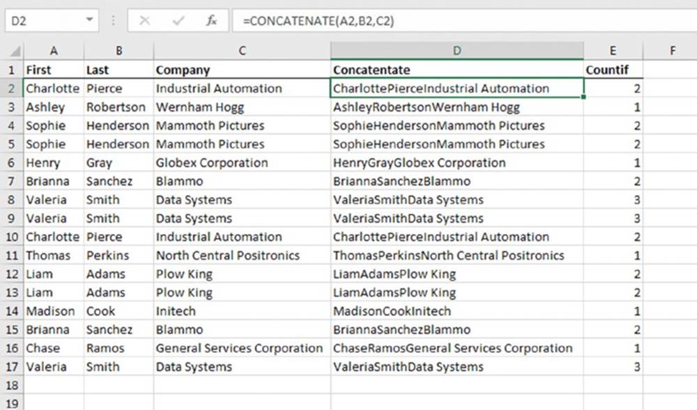
Figure 16.6 Using formulas to identify duplicate rows.
Splitting text
When importing data, you might find that multiple values are imported into a single column. Figure 16.7 shows an example of this type of import problem.
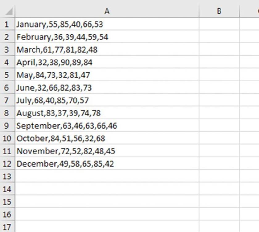
Figure 16.7 The imported data was put in one column rather than multiple columns.
If all the text is the same length (knows as a fixed-width text file), you might be able to write a series of formulas that extract the information to separate columns. The LEFT, RIGHT, and MID functions are useful for this task. (See Chapter 5.)
You should also be aware that Excel offers two nonformula methods to assist in splitting data so it occupies multiple columns: Text to Columns and Flash Fill.
Using Text to Columns
The Text to Columns command is a handy tool that can parse strings into their component parts.
First, make sure that the column that contains the data to be split up has enough empty columns to the right to accommodate the extracted data. Then select the data to be parsed and choose Data ➜ Data Tools ➜ Text to Columns.
Excel displays the Convert Text to Columns Wizard, which consists of a series of dialog boxes that walk you through the steps to convert a single column of data into multiple columns. Figure 16.8 shows the initial step, in which you choose the type of data:
§ Delimited: The data to be split is separated by delimiters such as commas, spaces, slashes, or other characters.
§ Fixed Width: Each component occupies the same number of characters.
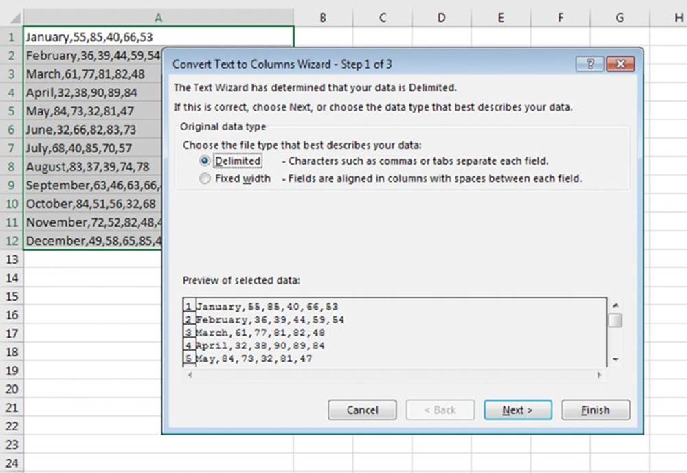
Figure 16.8 The first dialog box in the Convert Text to Columns Wizard.
Make your choice and click Next to move on to step 2, which depends on the choice you made in step 1.
If you’re working with delimited data, specify the delimiting character or characters (a comma in this example). You’ll see a preview of the result. If you’re working with fixed width data, you can modify the column breaks directly in the preview window. Click and drag the vertical lines to move the column break to another location. Single-click to add a new vertical line. Double-click an existing vertical line to remove it.
When you’re satisfied with the column breaks, click Next to move to step 3. In this step, you can click a column in the preview window and specify formatting for the column, or you can indicate that the column should be skipped. Click Finish, and Excel will split the data as specified. The original data will be replaced.
Using Flash Fill
The Text to Columns Wizard works well for many types of data, but sometimes you’ll encounter data that can’t be parsed by that wizard. For example, the Text to Columns Wizard is useless if you have variable width data that doesn’t have delimiters. In such a case, using the Flash Fill feature might save the day.
Flash Fill uses pattern recognition to extract data (and concatenate data). Just enter a few examples in a column that’s adjacent to the data and then choose Data ➜ Data Tools ➜ Flash Fill (or press Ctrl+E). Excel analyzes the examples and attempts to fill in the remaining cells. If Excel didn’t recognize the pattern you had in mind, press Ctrl+Z, add another example or two, and try again.
Figure 16.9 shows a worksheet with some text in a single column. The goal is to extract the number from each cell and put it into a separate cell. The Text to Columns Wizard can’t do it because the space delimiters aren’t consistent. You could write an array formula, but it would be complicated. Another option is to write a custom worksheet function using VBA. This might be a good job for Flash Fill.
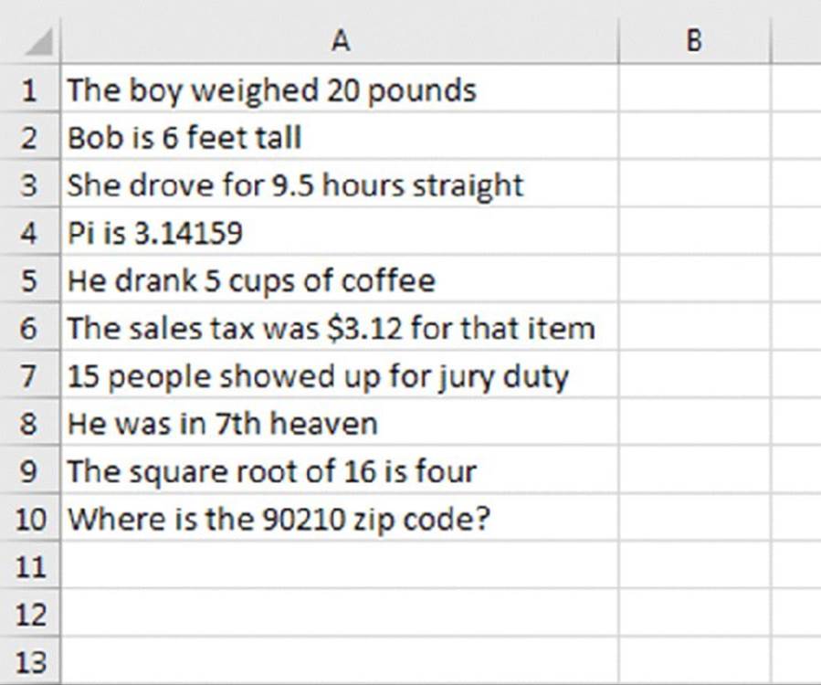
Figure 16.9 The goal is to extract the numbers in column A.
To try using Flash Fill, select cell B1 and type the first number (20). Move to B2 and type the second number (6). Can Flash Fill identify the remaining numbers and fill them in? Choose Data ➜ Data Tools ➜ Flash Fill (or press Ctrl+E), and Excel fills in the remaining cells in a flash. Figure 16.10 shows the result.
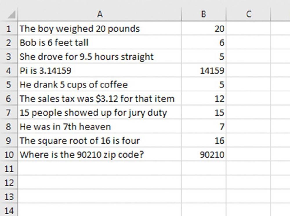
Figure 16.10 Using manually entered examples in B1 and B2, Excel makes some incorrect guesses.
It looks good. Excel somehow managed to extract the numbers from the text. Examine the results more closely, though, and you see that it failed for numbers that include decimal points. Accuracy increases if you provide more examples—such as an example of a decimal number. Delete the suggested values, enter 3.12 into cell B6, and press Ctrl+E. This time, Excel gets them all correct (see Figure 16.11).
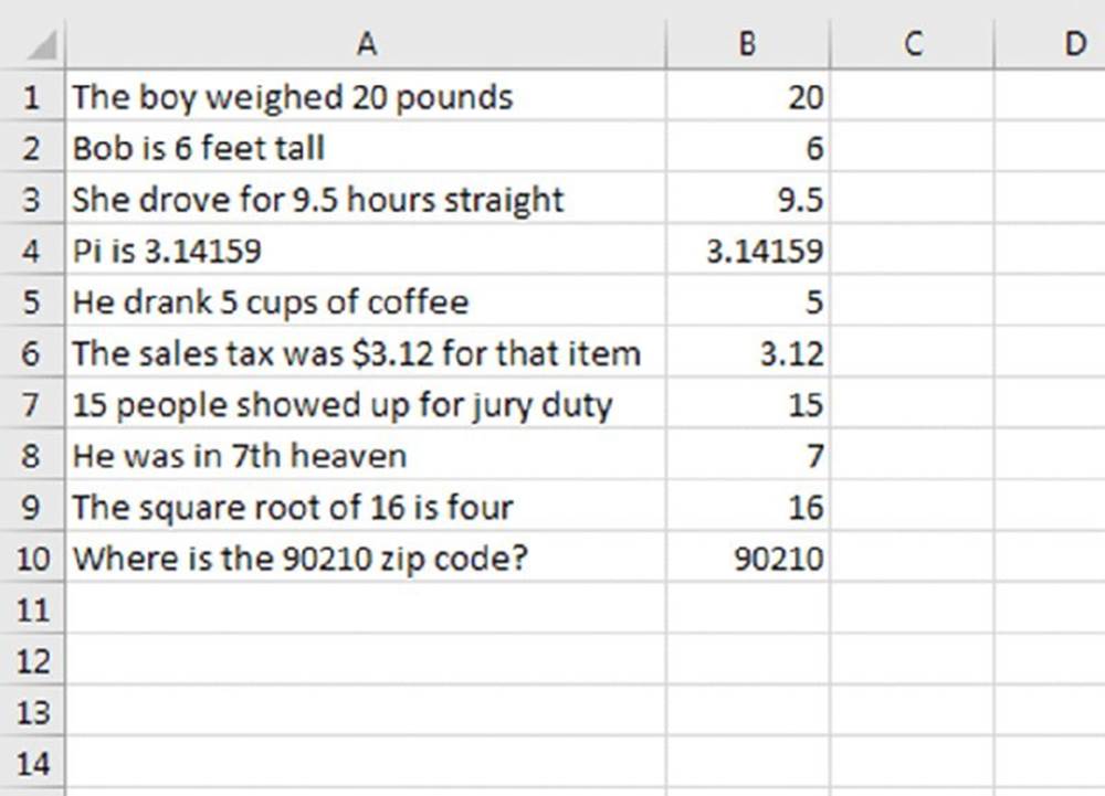
Figure 16.11 After entering an example of a decimal number, Excel gets them all correct.
This simple example demonstrates two important points:
§ You must examine your data carefully after using Flash Fill. Just because the first few rows are correct, you can’t assume that Flash Fill worked correctly for all rows.
§ Flash Fill increases accuracy when you provide more examples.
Figure 16.12 shows another example: names in column A. The goal is to use Flash Fill to extract the first, last, and middle name (if it has one). In column B, Flash Fill works great if you give it only two examples (Mark and Tim). Plus, it successfully extracts all the last names, using Russell and Colman as examples. Flash Fill has trouble extracting the middle names if some of the names have them and some don’t. In that case you can use the following formula to get the middle name or initial:
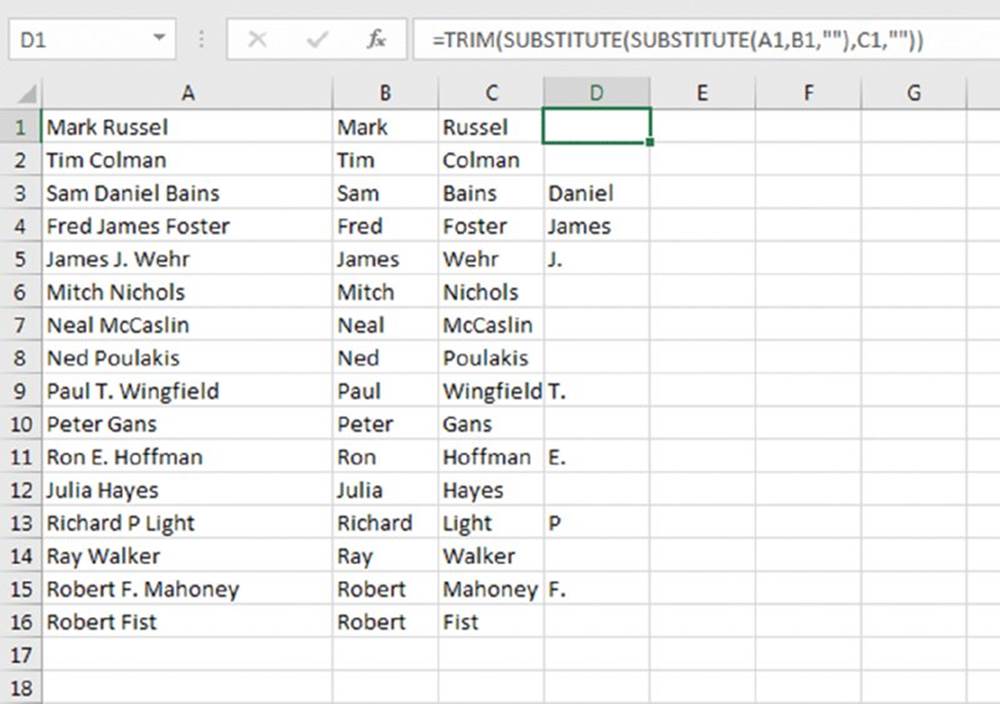
Figure 16.12 Using Flash Fill to split names.
=TRIM(SUBSTITUTE(SUBSTITUTE(A1,B1,""),C1,""))
The inner SUBSTITUTE replaces the first name with an empty string, the outer SUBSTITUTE replaces the last name with an empty string, and the TRIM function removes any extra spaces.
![]() Cross-Ref
Cross-Ref
See Chapter 5 for a formula-based solution for splitting names.
In addition to clicking the Flash Fill button on the Data tab of the Ribbon or using the Ctrl+E shortcut, Excel may recognize that you’re attempting to extract data and suggest an extraction as you type. Figure 16.13 shows Excel’s Flash Fill suggestion after typingMark in cell B1 and the first two letters of Tim in B2.
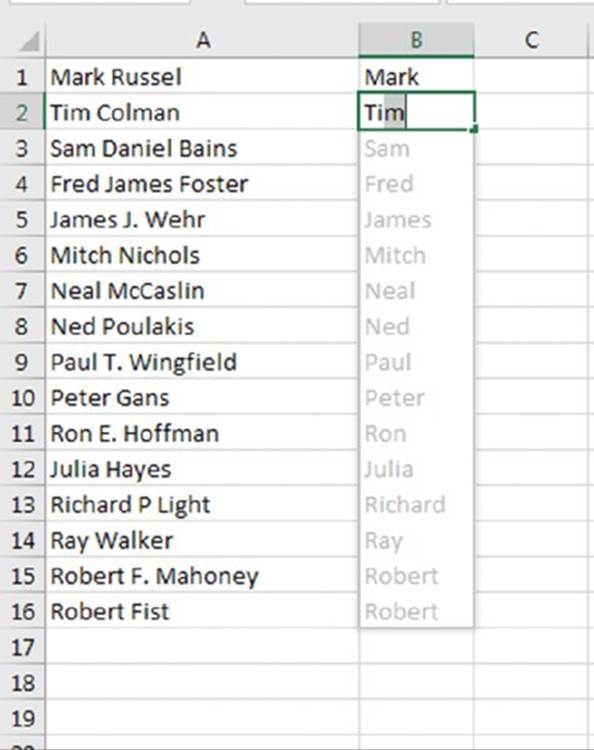
Figure 16.13 Excel suggests a Flash Fill as you type.
At this point, pressing the down arrow will complete the Flash Fill. Note that if you type the entire name, Tim, the suggestion goes away. You can simply move to the next cell and begin typing that name to get the suggestions to show again.
Here’s another example of using Flash Fill. Say you have a list of URLs and need to extract the domain (the part of the URL that ends in .com, .net, and so on).
Figure 16.14 shows a list of URLs. Flash Fill required just two examples of the domain entered into column B. As we typed 31engine in cell B2, Flash Fill suggested the remaining rows and we pressed the down arrow to fill them.
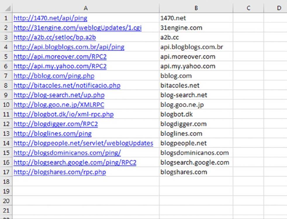
Figure 16.14 Using Flash Fill to extract domains from URLs.
Unlike formulas, Flash Fill is not dynamic. That is, if your data changes, the flash-filled column does not update.
Flash Fill seems to work reliably if the data is consistent, but it’s still a good idea to examine the results carefully. And think twice before trusting Flash Fill with important data. There’s no way to document how the data was extracted. You just have to trust Excel.
![]() Note
Note
You can also use the Flash Fill feature to create new data from multiple columns. Just provide a few examples of how you want the data combined, and Excel will figure out the pattern and fill in the column.
Changing the case of text
Often, you’ll want to make text in a column consistent in terms of case. Excel provides no direct way to change the case of text, but it’s easy to do with formulas. See the sidebar “Transforming data with formulas.”
The three relevant functions are
§ UPPER: Converts the text to ALL UPPERCASE.
§ LOWER: Converts the text to all lowercase.
§ PROPER: Converts the text to Proper Case. (The first letter in each word is capitalized, as in a proper name.)
These functions are quite straightforward. They operate only on alphabetic characters. They ignore all other characters and return them unchanged.
If you use the PROPER function, you’ll probably need to do some additional cleanup to handle exceptions. Here are some examples of transformations that you’d probably consider incorrect:
§ The letter following an apostrophe is always capitalized (for example, Don’T). This is done, apparently, to handle names like O’Reilly.
§ The PROPER function doesn’t handle names with an embedded capital letter, such as McDonald.
§ “Minor” words—such as and and the—are always capitalized. For example, some would prefer that the third word in United States Of America not be capitalized.
You can correct some of these problems by using Find and Replace.
![]() Transforming data with formulas
Transforming data with formulas
Many of the data cleanup examples in this chapter describe how to use formulas and functions to transform data in some way. For example, you can use the UPPER function to transform text into uppercase. When the data is transformed, you’ll have two columns: the original data and the transformed data. Almost always, you’ll want to replace the original data with the transformed data. Here’s how:
1. Insert a new temporary column for formulas to transform the original data.
2. Create your formulas in the temporary column and make sure that the formulas do what they were intended to do.
3. Select the formula cells.
4. Choose Home ➜ Clipboard ➜ Copy (or press Ctrl+C).
5. Select the original data cells.
6. Choose Home ➜ Clipboard ➜ Paste ➜ Values (V).
This procedure replaces the original data with the transformed data. Then you can delete the temporary column that holds the formulas.
Removing extra spaces
It’s usually a good idea to ensure that data doesn’t have extra spaces. It’s impossible to spot a space character at the end of a text string. Extra spaces can cause lots of problems, especially when you need to compare text strings. The text July is not the same as the text July with a space appended to the end. The first is four characters long, and the second is five characters long.
Create a formula that uses the TRIM function to remove all leading and trailing spaces, and replace multiple spaces with a single space. This example uses the TRIM function. The formula returns Fourth Quarter Earnings (with no excess spaces):
=TRIM(" Fourth Quarter Earnings ")
Data that is imported from a web page often contains a different type of space: a nonbreaking space, indicated by   in HTML code. In Excel, this character can be generated by this formula:
=CHAR(160)
You can use a formula like this to replace those spaces with normal spaces:
=SUBSTITUTE(A2,CHAR(160)," ")
Or use this formula to replace the nonbreaking space character with normal spaces and remove excess spaces:
=TRIM(SUBSTITUTE(A2,CHAR(160)," "))
Removing strange characters
Often, data imported into an Excel worksheet contains strange (often unprintable) characters. You can use the CLEAN function to remove all nonprinting characters from a string. If the data is in cell A2, this formula will do the job:
=CLEAN(A2)
![]() Note
Note
The CLEAN function can miss some nonprinting Unicode characters. This function is programmed to remove the first 32 nonprinting characters in the 7-bit ASCII code. Consult the Excel Help system for information on how to remove the nonprinting Unicode characters. (Search Help for the CLEAN function.)
Converting values
You may need to convert values from one system to another. For example, you may import a file that has values in fluid ounces, but those values need to be expressed in milliliters. Excel’s handy CONVERT function can perform that and many other conversions.
If cell A2 contains a value in ounces, the following formula converts it to milliliters.
=CONVERT(A2,"oz","ml")
This function is extremely versatile and can handle most common measurement units.
![]() Cross-Ref
Cross-Ref
See Chapter 10, “Miscellaneous Calculations,” for more information about the CONVERT function.
Excel can also convert between number bases. You may import a file that contains hexadecimal values, and you need to convert them to decimal. Use the HEX2DEC function to perform this conversion. For example, the following formula returns 1,279, which is the decimal equivalent of its hex argument:
=HEX2DEC("4FF")
Excel can also convert from binary to decimal (BIN2DEC) and from octal to decimal (OCT2DEC).
Functions that convert from decimal to another number base are DEC2HEX, DEC2BIN, and DEC2OCT.
![]() Note
Note
The BASE function, introduced in Excel 2013, converts a decimal number to any number base. Note that there is not a function that works in the opposite direction. Excel does not provide a function that converts any number base to decimal. You’re limited to binary, octal, and hexadecimal.
Classifying values
Often, you may have values that need to be classified into a group. For example, if you have ages of people, you might want to classify them into groups such as 17 or younger, 18 to 24, 25 to 34, and so on.
The easiest way to perform this classification is with a lookup table. Figure 16.15 shows ages in column A and classifications in column B. Column B uses the lookup table in D2:E9. The formula in cell B2 is
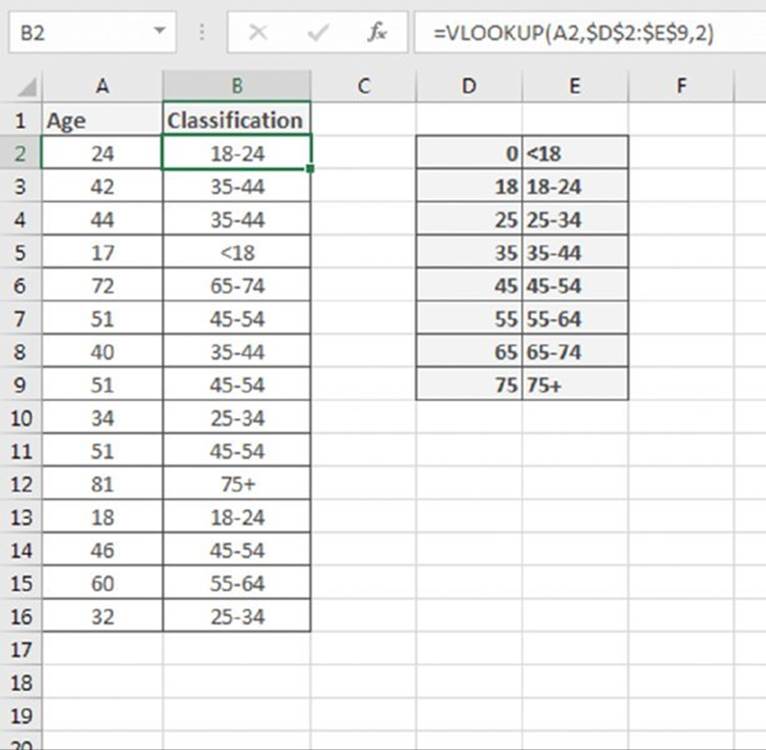
Figure 16.15 Using a lookup table to classify ages into age ranges.
=VLOOKUP(A2,$D$2:$E$9,2)
This formula was copied to the cells below.
You can also use a lookup table for nonnumeric data. Figure 16.16 shows a lookup table that is used to assign a region to a state.
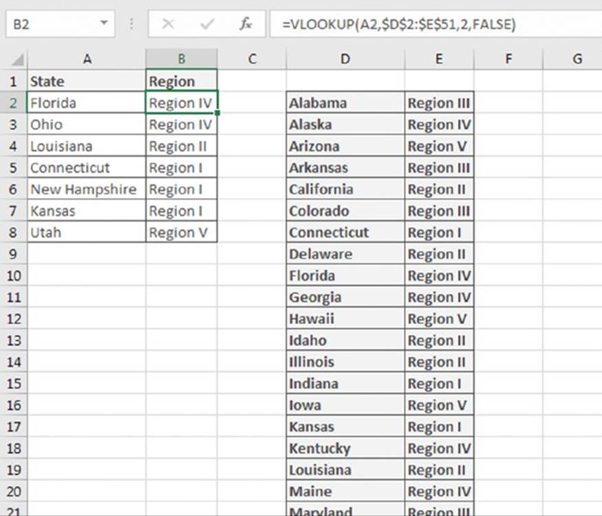
Figure 16.16 Using a lookup table to assign a region for a state.
The two-column lookup table is in the range D2:E51. The formula in cell B2, which was copied to the cells below, is
=VLOOKUP(A2,$D$2:$E$51,2,FALSE)
![]() Tip
Tip
A side benefit is that the VLOOKUP function will return #N/A if an exact match is not found—a good way to spot misspelled states. Using FALSE as the last argument in the function indicates that an exact match is required.
Joining columns
To combine data in two more columns, you can usually use the concatenation operator (&) in a formula. For example, the following formula combines the contents of cells A1, B1, and C1:
=A1&B1&C1
Often, you’ll need to insert spaces between the cells, such as if the columns contain a title, first name, and last name. Concatenating using the preceding formula would produce something like Mr.ThomasJones. To add spaces (to produce Mr. Thomas Jones), modify the formula like this:
=A1&" "&B1&" "&C1
You can also use the Flash Fill feature to join columns without using formulas. Just provide an example or two in an adjacent column, and press Ctrl+E.
Rearranging columns
If you need to rearrange the columns in a worksheet, you can insert a blank column and then drag another column into the new blank column. But then the moved column leaves a gap, which you need to delete.
Here’s an easier way:
1. Click the column header of the column you want to move.
2. Choose Home ➜ Clipboard ➜ Cut.
3. Click the column header to the right of where you want the column to go.
4. Right-click and choose Insert Cut Cells from the shortcut menu that appears.
Repeat these steps until the columns are in the order you desire.
You can also move or copy columns by dragging them with your mouse. Select the entire column by clicking on the column header, and then click on the column border and drag. (The cursor turns into four arrows when you’re on the border.) Hold down the Ctrl key while you drag, and you create a copy of the column in the new location while the original column remains where it was. Hold down the Shift key while you drag to move the column and insert it where you drop, shifting all other columns to the right.
Randomizing the rows
If you need to arrange rows in random order, here’s a quick way to do it. In the column to the right of the data, insert this formula into the first cell and copy it down:
=RAND()
Then sort the data using this column. The rows will be in random order, and you can delete the column.
Matching text in a list
You may have some data that you need to check against another list. For example, you may want to identify rows in which data in a particular column appears in a different list. Figure 16.17 shows a simple example. The data is in columns A:C. The goal is to identify the rows in which the Member Num appears in the Resigned Members list, in column F. These rows can then be deleted.
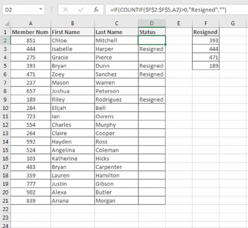
Figure 16.17 The goal is to identify member numbers that are in the resigned members list.
Here’s a formula entered into cell D2, and copied down, that will do the job:
=IF(COUNTIF($F$2:$F$5,A2)>0,"Resigned","" )
This formula displays the word Resigned if the Member Num in column A is found in the Resigned Members list. If the member number is not found, it returns an empty string. If the list is sorted by column D, the rows for all resigned members will appear together and can be quickly deleted.
This technique can be adapted to other types of list matching tasks.
Change vertical data to horizontal data
Figure 16.18 shows a common type of data layout that you might see when importing a file. Each record consists of three consecutive cells in a single column: Department, Name, and Location. The goal is to convert this data so that each record appears as a single row with three columns.
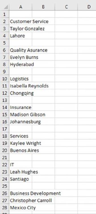
Figure 16.18 Vertical data that needs to be converted to three columns.
There are several ways to convert this type of data, but here’s a method that’s fairly easy. Start by creating column headers for Department, Name, and Location in row 1. In row 2, enter these four formulas as shown in Figure 16.19:
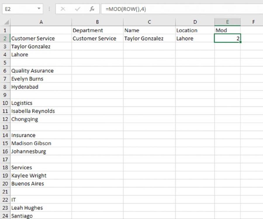
Figure 16.19 Use formulas to convert column data to row data.
B2: =A2
C2: =A3
D2: =A4
E2: =MOD(ROW(),4)
Copy the four formulas down as far as you have data. Each record is three pieces of data and a blank line. The MOD function returns the remainder when the row number is divided by four. All the rows with a 2 in the Mod column will be the ones you want to keep.
Copy columns B:E and choose Home ➜ Paste ➜ Values to convert the formulas to their values and delete column A. Select all the data and choose Sort from the Data tab on the Ribbon and sort on the Mod column (see Figure 16.20).
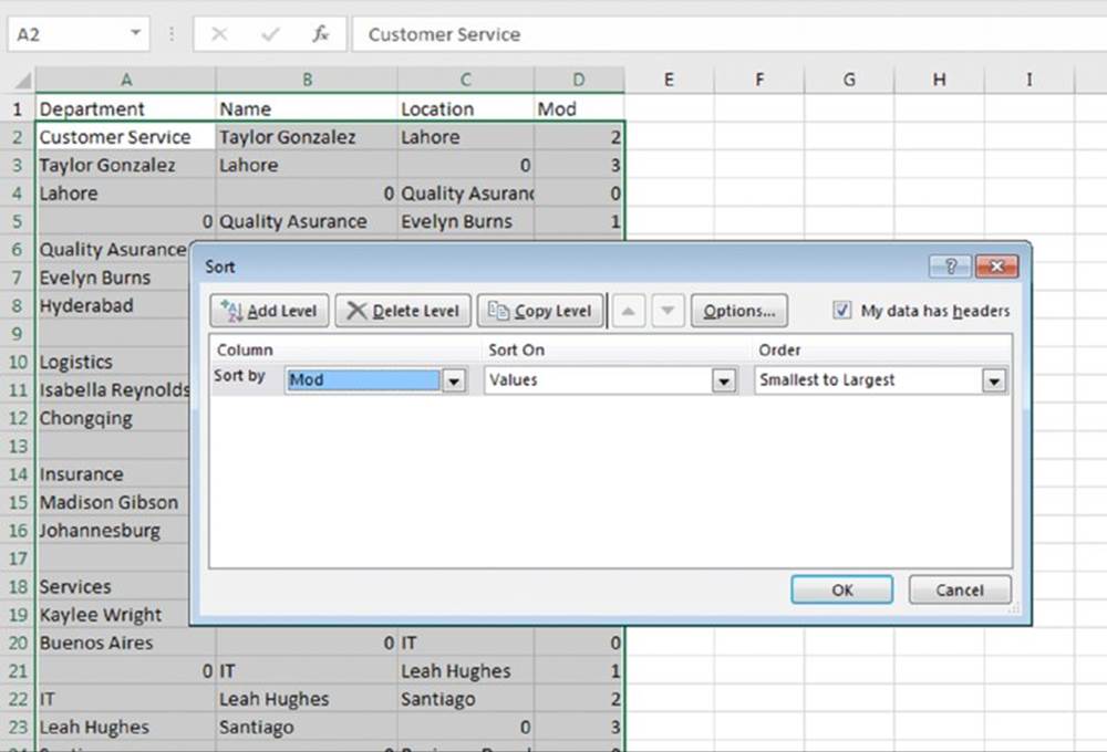
Figure 16.20 Sort the data on the Mod column to group the data.
Delete any rows that do not contain 2 in the Mod column, and you’re left with data in which each record is on its own row, as shown in Figure 16.21. You can now delete the Mod column.
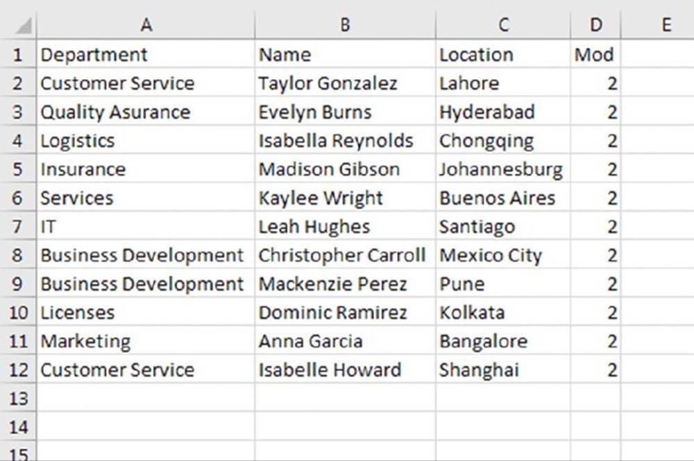
Figure 16.21 Each record of data is on its own row.
You can easily adapt this technique to work with vertical data that contains a different number of rows. Simply add as many formulas across as you need and change the second argument of the MOD function to the number of rows that represent one record.
Filling gaps in an imported report
When you import data, you can sometimes end up with a worksheet that looks something like the one shown in Figure 16.22. This type of report formatting is common. As you can see, an entry in column A applies to several rows of data. If you sort this type of list, the missing data messes things up, and you can no longer tell who sold what when.
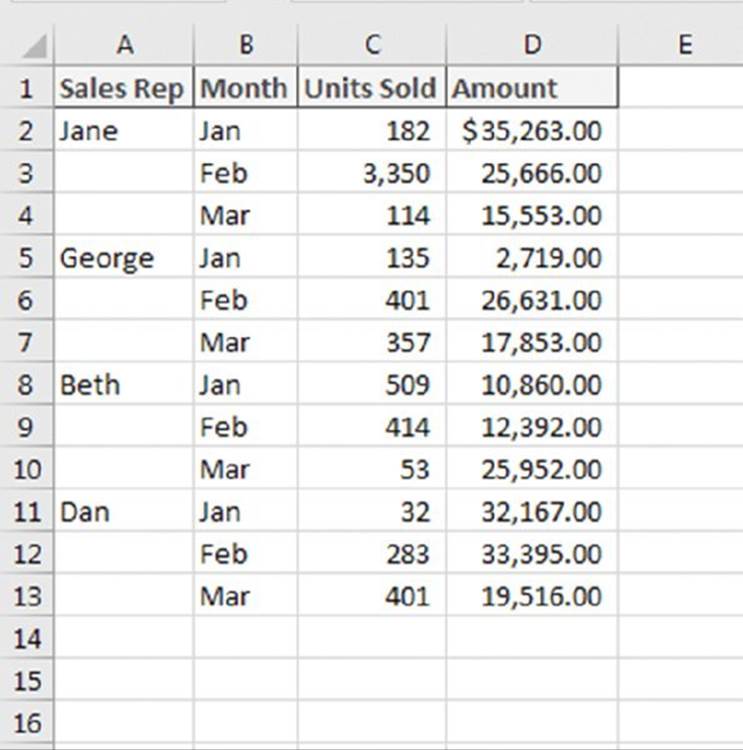
Figure 16.22 This report contains gaps in the Sales Rep column.
If the report is small, you can enter the missing cell values manually or by using a series of Home ➜ Editing ➜ Fill ➜ Down commands (or its Ctrl+D shortcut). If you have a large list that’s in this format, here’s a better way:
1. Select the range that has the gaps (A2:A13, in this example).
2. Choose Home ➜ Editing ➜ Find & Select ➜ Go to Special to display the Go to Special dialog box.
3. In the Go to Special dialog box, select the Blanks option and click OK. This action selects the blank cells in the original selection.
4. In the formula bar, type an equal sign (=) followed by the address of the first cell with an entry in the column (=A2, in this example), and then press Ctrl+Enter. Figure 16.23 shows the blank cells filled in.
5. Reselect the original range and press Ctrl+C to copy the selection.
6. Choose Home ➜ Clipboard ➜ Paste ➜ Paste Values to convert the formulas to values.
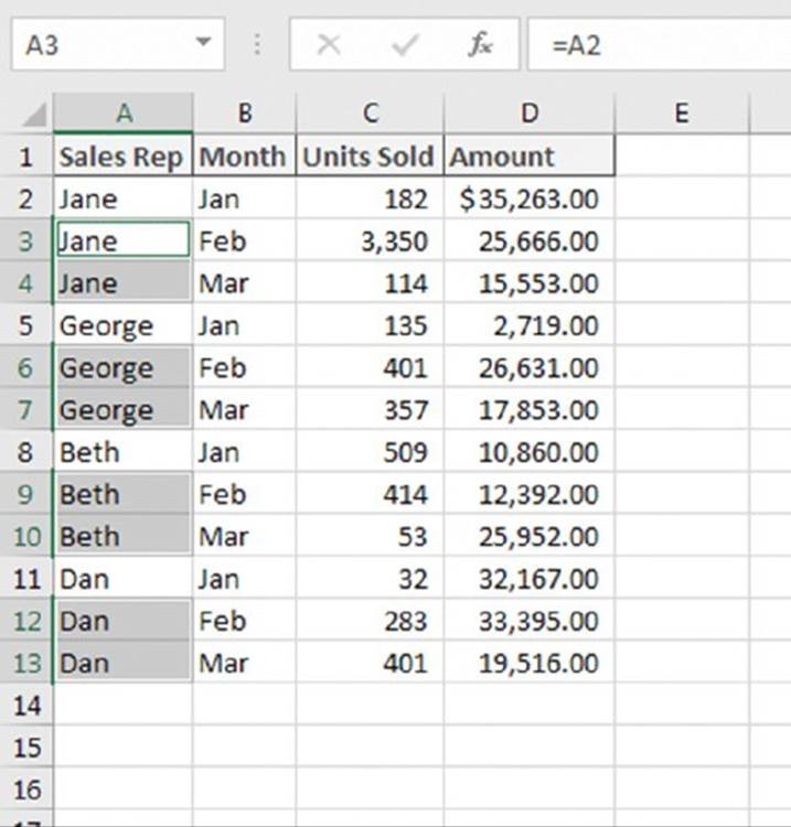
Figure 16.23 The gaps are gone, and this list can now be sorted.
After you complete these steps, the gaps are filled in with the correct information.
Spelling checking
If you use a word processing program, you probably take advantage of its spelling checker feature. Spelling mistakes can be embarrassing when they appear in a text document, but they can cause serious problems when they occur within your data. For example, if you tabulate data by month using a pivot table, a misspelled month name will make it appear that a year has 13 months.
To access the Excel spell checker, choose Review ➜ Proofing ➜ Spelling or press F7. To check the spelling in just a particular range, select the range before you activate the spell checker.
If the spell checker finds any words that it does not recognize as correct, it displays the Spelling dialog box. Figure 16.24 shows the Spelling dialog box where you can ignore the misspelling, change it to a suggested spelling, or add the word to the dictionary.
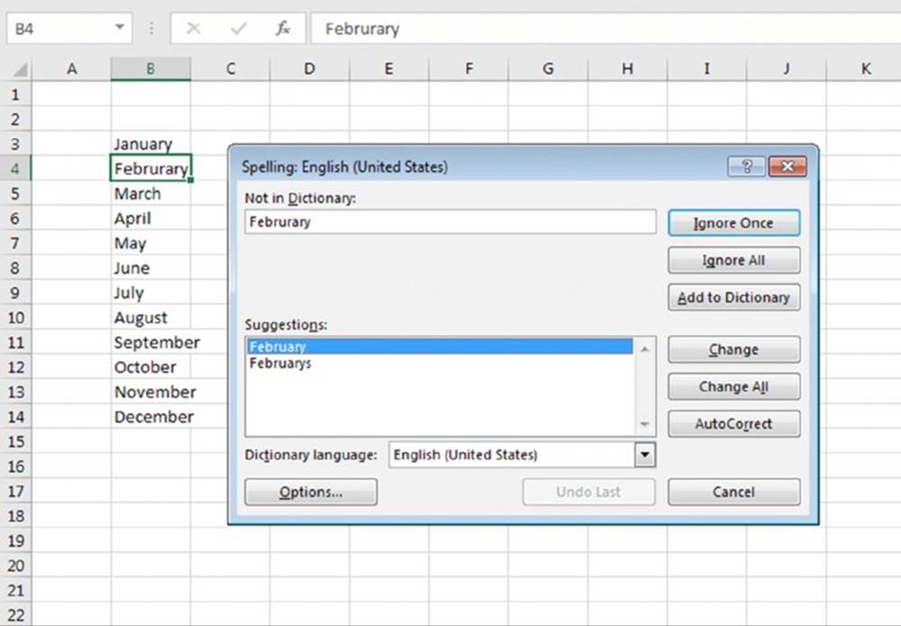
Figure 16.24 Misspelled words can be ignored or changed.
Replacing or removing text in cells
You may need to systematically replace (or remove) certain characters in a column of data. For example, you may need to replace all backslash characters with forward slash characters. In many cases, you can use Excel’s Find and Replace dialog box to accomplish this task. To remove text using the Find and Replace dialog box, just leave the Replace With field empty.
In other situations, you may need a formula-based solution. Consider the data shown in Figure 16.25. The goal is to replace the second hyphen character with a colon. Using Find and Replace wouldn’t work because there’s no way to specify that only the second hyphen should be replaced.
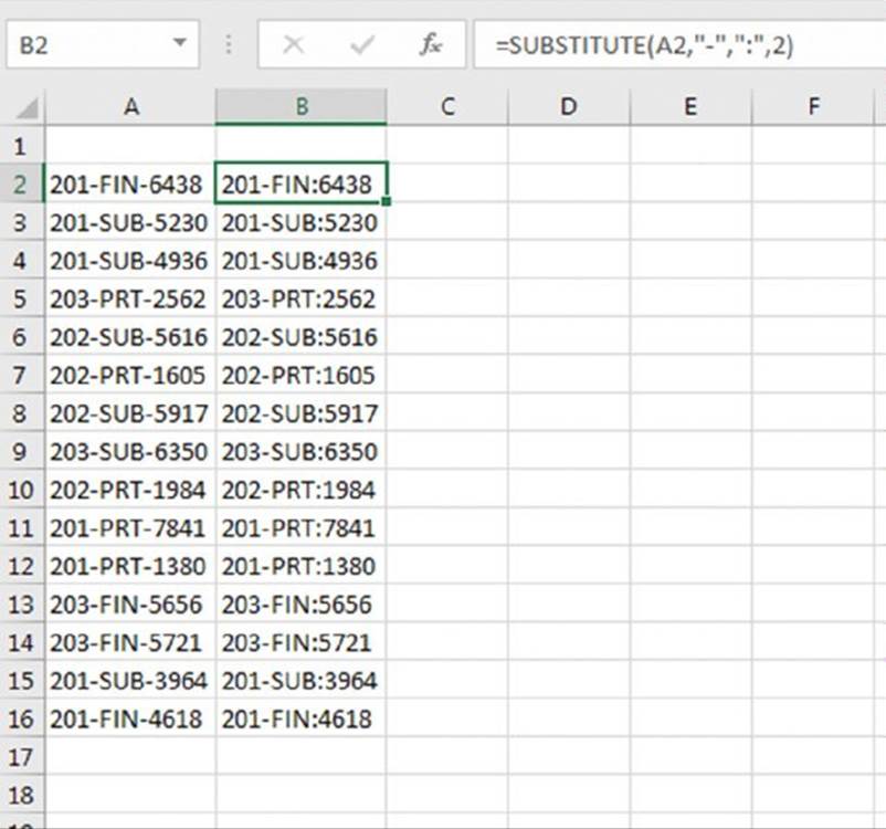
Figure 16.25 To replace only the second hyphen in these cells, Find and Replace is not an option.
In this case, the solution is a fairly simple formula that replaces the second occurrence of a hyphen with a colon:
=SUBSTITUTE(A2,"-",":",2)
To remove the second occurrence of a hyphen, just omit the third argument for the SUBSTITUTE function:
=SUBSTITUTE(A2,"-",,2)
This is another example in which Flash Fill can also do the job.
![]() Note
Note
If you’ve worked with programming languages, you may be familiar with the concept of regular expressions. A regular expression is a way to match strings of text using concise (and often confusing) codes. Excel does not support regular expressions, but if you search the Web, you’ll find ways to incorporate regular expressions in VBA, plus a few add-ins that provide this feature in the workbook environment.
Adding text to cells
If you need to add text to a cell, the only solution is to use a new column of formulas. Here are some examples.
This formula adds: “ID: ” to the beginning of a cell:
="ID: "&A2
This formula adds “.mp3” to the end of a cell:
=A2&".mp3"
This formula inserts a hyphen after the third character in a cell:
=LEFT(A2,3)&"-"&RIGHT(A2,LEN(A2)–3)
You can also use Flash Fill to add text to cells.
Fixing trailing minus signs
Imported data sometimes displays negative values with a trailing minus sign. For example, a negative value may appear as 3,498- rather than the more common -3,498. Excel does not convert these values. In fact, it considers them to be nonnumeric text.
The solution is so simple it may even surprise you:
1. Select the data that has the trailing minus signs. The selection can also include positive values.
2. Choose Data ➜ Data Tools ➜ Text to Columns.
3. When the Text to Columns dialog box appears, click Finish.
This procedure works because of a default setting in the Advanced Text Import Settings dialog box (which you don’t even see, normally). To display this dialog box, shown in Figure 16.26, go to step 3 in the Text to Columns Wizard dialog box and click Advanced.
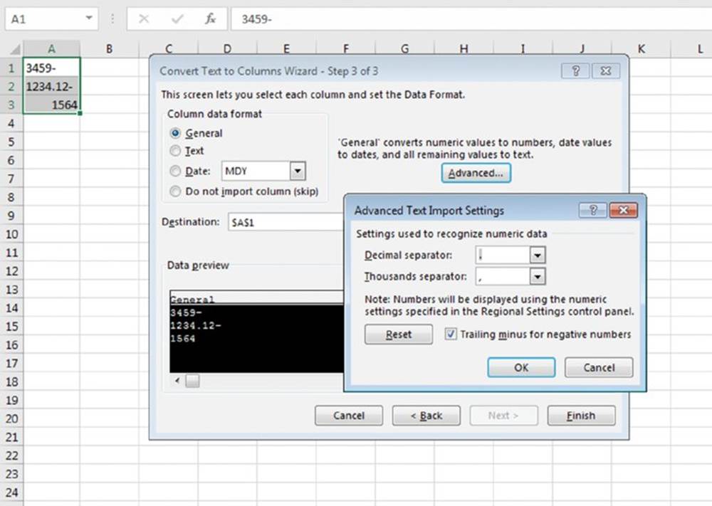
Figure 16.26 The Trailing Minus for Negative Numbers option makes it easy to fix trailing minus signs in a range of data.
Or you can use Flash Fill to fix the trailing minus signs. If the range contains positive values, you may need to provide several examples.
A Data Cleaning Checklist
This section contains a list of items that could cause problems with data. Not all these are relevant to every set of data:
§ Does each column have a unique and descriptive header?
§ Is each column of data formatted consistently?
§ Did you check for duplicate or missing rows?
§ For text data, are the words consistent in terms of case?
§ Does the data include any unprintable characters?
§ Did you check for spelling errors?
§ Does the data contain extra spaces?
§ Are the columns arranged in the proper (or logical) order?
§ Are any cells blank that shouldn’t be?
§ Did you correct any trailing minus signs?
§ Are the columns wide enough to display all data?
Exporting Data
This chapter began with a section on importing data, so it’s only appropriate to end it with a discussion of exporting data to a file that’s not a standard Excel file.
Exporting to a text file
When you choose File ➜ Save As, the Save As dialog box offers you a variety of text file formats. The three types are
§ CSV: Comma-separated value files
§ TXT: Tab-delimited files
§ PRN: Formatted text
I discuss these files types in the sections that follow.
CSV files
When you export a worksheet to a CSV file, the data is saved as displayed. In other words, if a cell contains 12.8312344 but is formatted to display with two decimal places, the value will be saved as 12.83.
Cells are delimited with a comma character, and rows are delimited with a carriage return and line feed.
![]() Note
Note
If you export a file using the Macintosh variant, rows are delimited with a carriage return only (no line feed character).
Note that if a cell contains a comma, the cell value is saved within quotation marks. If a cell contains a quotation mark character, that character appears twice.
TXT files
Exporting a workbook to a TXT file is almost identical to the CSV file format described earlier. The only difference is that cells are separated by a tab character instead of a comma.
If your worksheet contains any Unicode characters, you should export the file using the Unicode variant. Otherwise, Unicode characters will be saved as question mark characters.
PRN files
A PRN file is much like a printed image of the worksheet. The cells are separated by multiple space characters. Also, a line is limited to 240 characters. If a line exceeds that limit, the remainder appears on the next line. PRN files are rarely used.
Exporting to other file formats
Excel also lets you save your work in several other formats:
§ Data Interchange Format: These files have a DIF extension. Not used very often.
§ Symbolic Link: These files have an SYLK extension. Not used very often.
§ Portable Document Format: These files have a PDF extension. This is a common “read-only” file format.
§ XML Paper Specification Document: These files have an XPS extension; they’re Microsoft’s alternative to PDF files. Not used very often.
§ Web Page: These files have an HTM extension. Often, saving a file as a web page generates a directory of ancillary files required to render the page accurately.
§ OpenDocument Spreadsheet: These files have an ODS extension. They are compatible with various open source spreadsheet programs.
All materials on the site are licensed Creative Commons Attribution-Sharealike 3.0 Unported CC BY-SA 3.0 & GNU Free Documentation License (GFDL)
If you are the copyright holder of any material contained on our site and intend to remove it, please contact our site administrator for approval.
© 2016-2026 All site design rights belong to S.Y.A.