My Excel 2016 (2016)
7. Advanced Formatting
In this chapter, you’ll find out how to set up formatting that changes as the data changes. You’ll see how you can use themes to provide consistency in design between workbooks. Topics in this chapter include the following:
→ Creating custom number formats
→ Emphasizing the top 10
→ Highlighting duplicate values in a list
→ Ensuring consistency with themes and cell styles
→ Creating hyperlinks
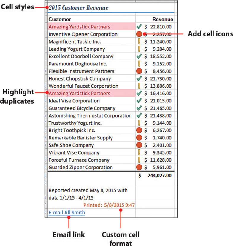
Custom formats allow you to create your own number formats, such as including text in a cell but still allowing calculations. With conditional formatting, you can apply a variety of formatting to data that automatically changes as the data updates. You can also design your own styles and themes to keep a consistent look among your workbooks.
Creating Custom Number Formats
Despite all the number formats available, not all the possible situations are covered. For example, you may need to add a K to show thousands in a cell. However, you can’t actually have the text in the cell because it would interfere with calculations. That’s why there’s the option of custom formats, allowing you to create a format specific to your situation.
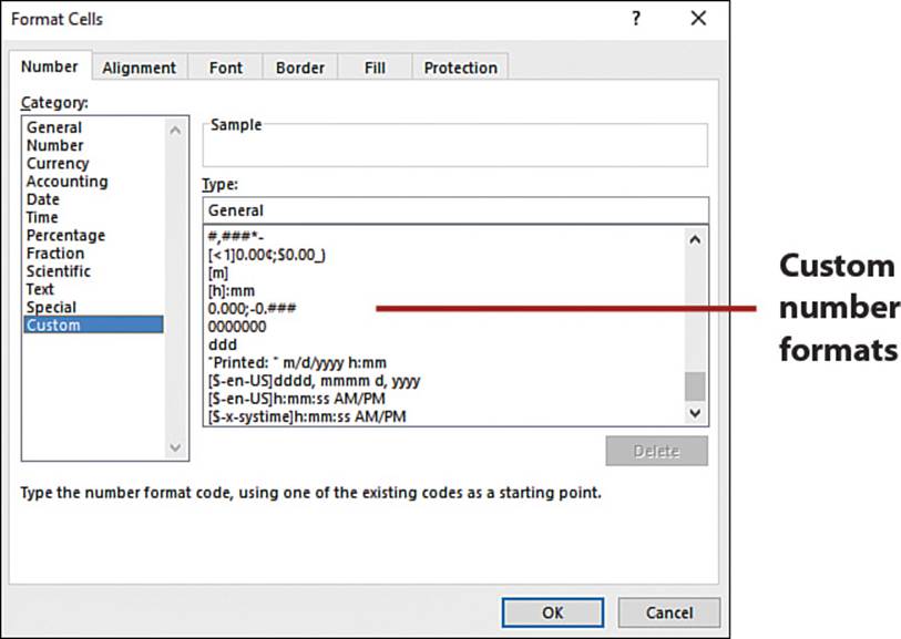
Once you’ve created a custom number format, you can apply it to any cell in the workbook, just like a built-in number format. Custom number formats are found under the Custom category of the Format Cells dialog box. The newest custom number format is found at the bottom of the Type list.
Sharing Custom Formats
Custom formats are saved with the workbook they are created in. To share the format, copy a cell with the format and paste it in the other workbook.
The Four Sections of a Custom Number Format
A custom format can contain up to four different sections, each separated by a semicolon: positive; negative; zero; text.
Each section can have its own format rules, and you don’t have to include all the sections in your custom format. If you specify only two sections, the first section is used for positive numbers and zeros, and the second section is used for negative numbers. If there is only one section, it’s used for all numbers. To skip a section but include one that follows it, you must include the ending semicolon for the section you skipped.
Optional Versus Required Digits
Use the pound (#) sign as a placeholder if you would like to display a certain number of characters that are not necessary. If the numbers are required, use zeros instead.
1. Select the range you want to format.
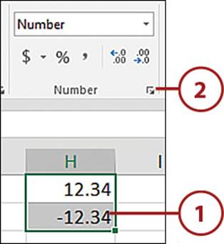
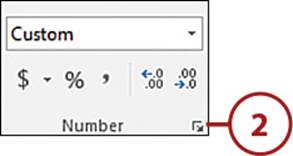
2. From the Home tab, select the Number group’s dialog box launcher.
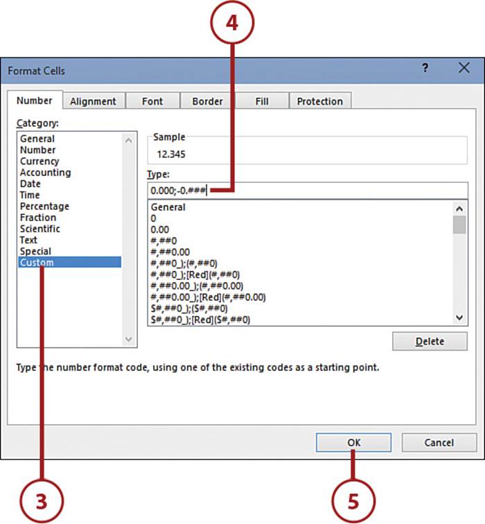
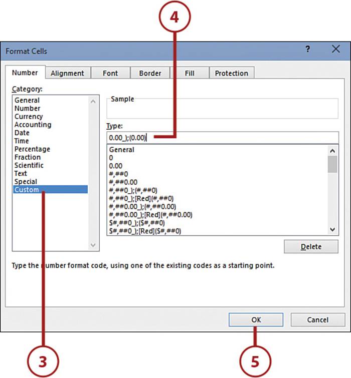
3. On the Number tab, select the Custom category.
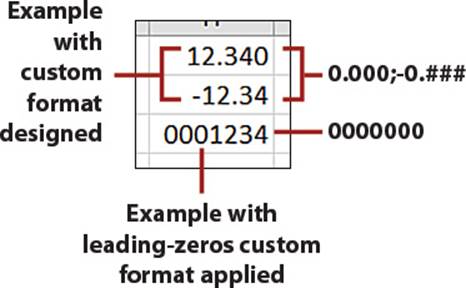
4. In the Type field, replace the existing entry with the following to format the positive section to always show three decimal places and the negative section to show only what’s entered:
0.000;-0.###
5. Click OK.
Preserve Leading Zeros
When you enter a number starting with a zero, Excel drops the leading zero. You can format the cell as text, but what if you forget to type the zero? Enter the following to ensure seven values to the left of the decimal:
0000000
Use the Thousands Separator, Color Codes, and Text
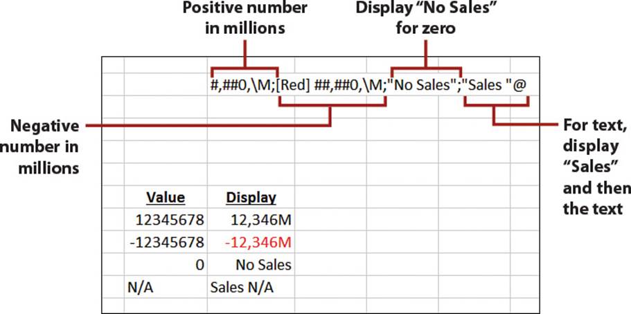
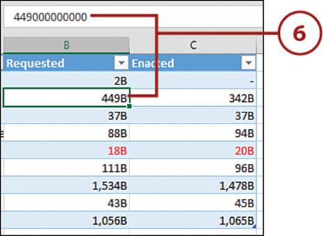
When you have large numbers, one way to make them more readable is to include a thousands separator (usually a comma). Another is to scale the number so that thousands, millions, or billions are represented by letters. For example, 2,000,000 could be shown as 2B.
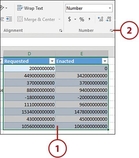
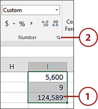
1. Select the range you want to format.
2. From the Home tab, select the Number group’s dialog box launcher.
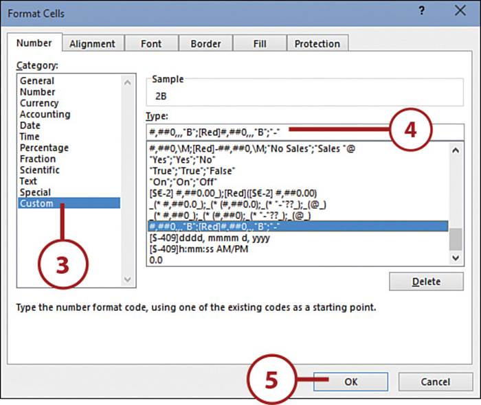
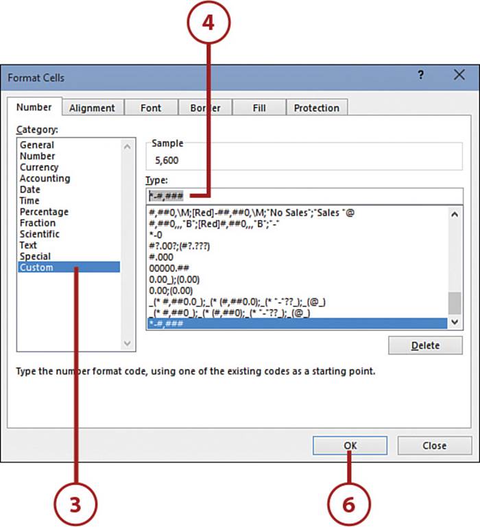
3. On the Number tab, select the Custom category.
4. In the Type box, enter the following:
#,##0,,,”B”;[Red]#,##0,,,”B”;”-”
Custom Format Explanation
This custom format will remove the nine rightmost digits from the value and add a B at the end, symbolizing billions. In the negative portion of the format, the unary symbol (minus sign) is not used. Instead, the [Red] code colors the negative number red. In the zero portion of the format, a dash will be shown instead of a zero. The text portion is not used.
5. Click OK.
6. The custom format is applied to the range, but the original values are retained in the cell.
>>>Go Further: Format Options in Detail
To include a thousands separator, use a comma in the format, such as #,###.0. To scale a number by thousands (for example, to show 22,000 as 22), include a comma at the end of the numeric format for each multiple of 1,000 (#,##0,).
You can use eight text color codes in a format: red, blue, green, yellow, cyan, black, white, and magenta. For other colors, you use numbered color codes (color1–color56). You place the color in square brackets, such as [cyan] or [color35]. The color should be the first element of a numeric formatting section.
To add text to a numeric format, place the characters in quotation marks. The following characters are an exception to this rule and do not require quotation marks:
: $ - + / ( ) : ! ^ & ‘ ~ { } = < > and the space character
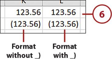
Line Up Decimals
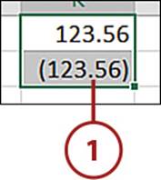
Use an underscore (_) in a format to make a character to the right of the underscore, such a parentheses, invisible in the cell but still take up space. You can use this formatting option to line up a column of positive and negative numbers.
1. Select the range you want to format.
2. From the Home tab, select the Number group’s dialog box launcher.
3. On the Number tab, select the Custom category.
4. Enter the following:
0.00_);(0.00)
5. Click OK.
6. The decimals of the positive and negative values in the column now line up.
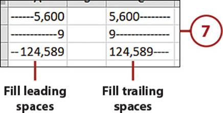
Fill Leading and Trailing Spaces
Instead of you typing in extra characters to fill the blank area in a cell, an asterisk (*) followed by a character will automatically display and adjust extra characters as the column is resized. As a bonus, the extra characters won’t interfere with calculations because they aren’t really in the cell.
1. Select the range you want to format.
2. From the Home tab, select the Number group’s dialog box launcher.
3. On the Number tab, select the Custom category.
4. In the Type box, enter *-#,### to fill leading spaces.
Or
5. Enter #,###-* to fill trailing spaces.
6. Click OK.
7. The extra character will fill the cell.
Show More Than 24 Hours in a Time Format
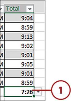
When you have time values greater than 24, Excel doesn’t seem to provide the proper answer. For example, you have a timesheet with daily start and end times for hours worked. You’ve calculated the hours worked each day and now you want to sum the entire month. But when you do, you get a value such as 7:26, which isn’t correct. The correct answer is there—it’s just a matter of formatting to see it.
1. Select the range you want to format.
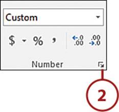
2. From the Home tab, select the Number group’s dialog box launcher.
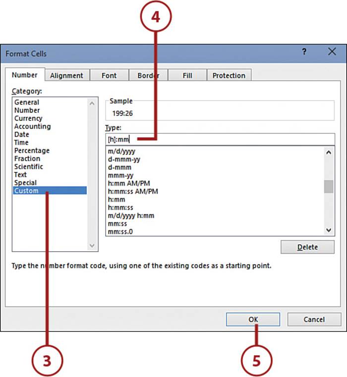
3. On the Number tab, select the Custom category.
4. Enter the following:
[h]:mm
5. Click OK.
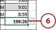
6. The correct total number of hours is shown.
>>>Go Further: Date and Time Code Options
Date and time formats have the greatest variety of codes available when it comes to creating number formats. There isn’t a real difference between the codes ## and ###; however, the difference between formatting a date cell mm or mmm is more obvious.
The following table lists the available date and time codes you can use when creating a format.
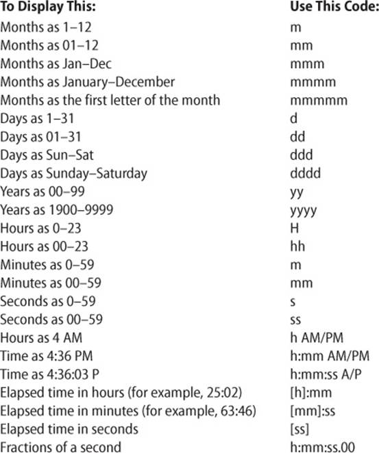
Here are a couple things to keep in mind when creating date and time formats:
• If the time format has an AM or PM in it, Excel bases the time on a 12-hour clock. Otherwise, Excel uses a 24-hour clock.
• When you’re creating a time format, the minutes code (m or mm) must appear immediately after the hour code (h or hh) or immediately before the seconds code (ss); otherwise, Excel displays months instead of minutes.
Creating Hyperlinks
Hyperlinks allow you to open web pages in your browser, create emails, and jump to a specific cell on a specific sheet in a specific workbook. For web and email addresses, Excel automatically recognizes what you’ve typed in and applies the format accordingly, turning the cell into a clickable link.
Create a Hyperlink to Another Sheet
Being able to create a hyperlink to a sheet can be useful if you want to create a table of contents for a large workbook or a series of workbooks.
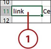
1. Select the cell where you want the link. It can contain the text you want to use as a hyperlink or it can be blank.
2. Click the Hyperlink button on the Insert tab.

Or
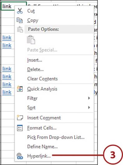
3. Right-click over the selection and select Hyperlink.
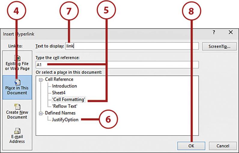
4. Click Place in This Document.
5. Select the sheet you want the link to jump to and enter the cell address you want selected.
Or
6. Select a range name from the Defined Names list.
7. Enter the text to display in the cell.
8. Click OK.
9. The link will appear blue and underlined.

Select a Hyperlink Cell to Edit or Remove
A link is triggered when you click it with the mouse. To select the cell without triggering it, use the keyboard arrow keys to navigate to the cell. You can then edit the cell, such as changing the font color.
To edit or remove a hyperlink, right-click the link and select Edit Hyperlink or Remove Hyperlink. When you remove the hyperlink, the text remains in the cell.
>>>Go Further: Link to Other Files
Links can be created to other workbooks and other file types, such as Word documents. You can even create a new file from scratch.
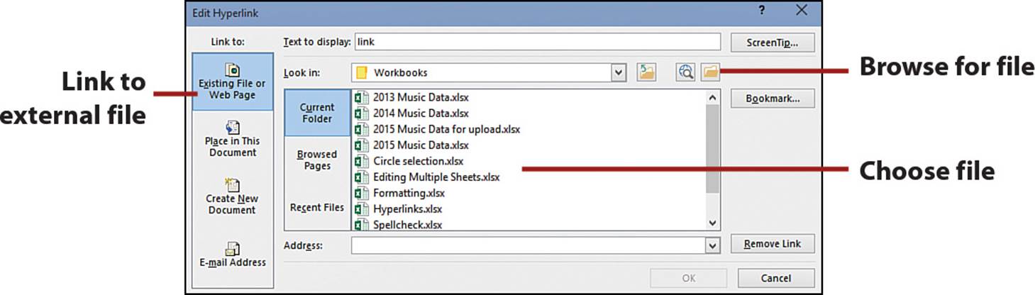
Click Existing File or Web Page in the Insert Hyperlink or Edit Hyperlink dialog box to link to another file. You can choose the file from a list or browse to it. When the user clicks the link, the file will open in its parent application. For example, if link is to a Word document, Word will open.
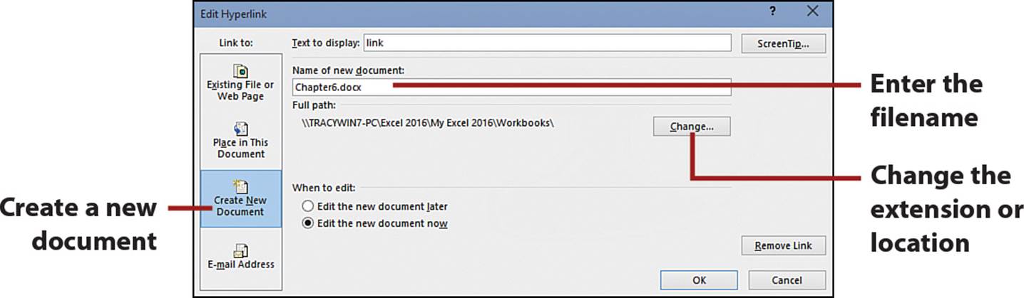
Click Create New Document in the Insert Hyperlink or Edit Hyperlink dialog box to create a new file and link to it. You can enter the filename with extension or click Change to open the Create New Document dialog box. This dialog box allows you to choose an extension from the Save As Type drop-down, choose a new file location, and enter the filename.
Link to a Web Page
You can add a link that opens a web page in the user’s default web browser.
Create a Simple Link
You can create a simple link by typing the web address directly in a cell, such as www.tsyrstad.wordpress.com. When Excel see’s the www, it knows it’s a web page, and once you press Enter, it converts the text to a link. But if you want to hide the address and have some other text appear in the cell instead, you must use the Hyperlink dialog box.
1. Select the cell where you want the link.
2. Click the Hyperlink button on the Insert tab.

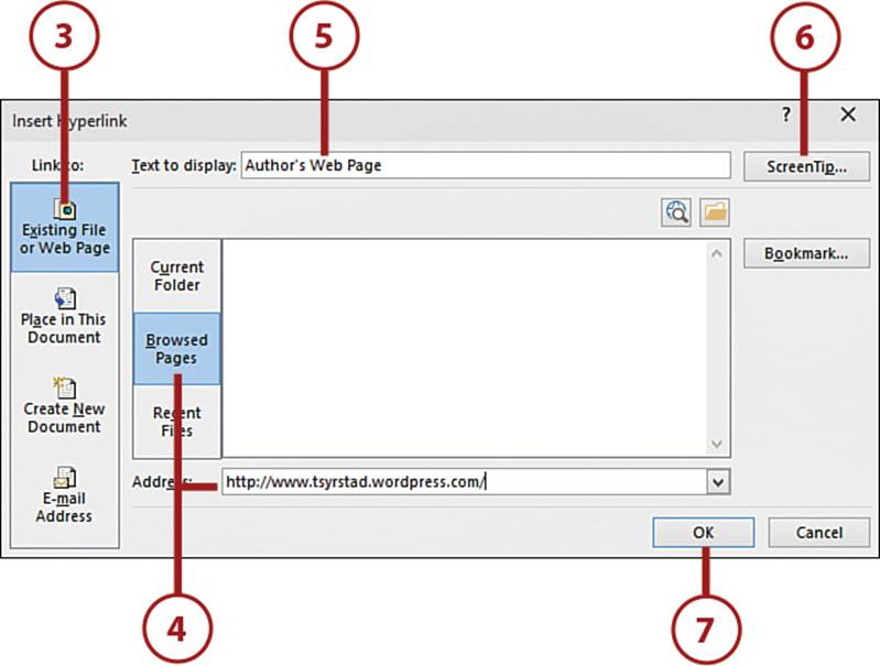
3. Click Existing File or Web Page.
4. Click Browsed Pages. Select from the list or enter a new address.
5. Enter the text to display in the cell.
6. If you want, enter a ScreenTip to appear when the pointer is over the link.
7. Click OK.
8. The link will appear blue and underlined.

Dynamic Cell Formatting with Conditional Formatting
Conditional formatting allows you to apply formatting and icons that will automatically update as the data does. You can create your own formatting rule (see “Create a Custom Rule”) or use one of the predefined rules found on the Conditional Formatting drop-down.
Use Icons to Mark Data
You can use icons to mark how values compare to each other. For example, use a green check mark for values in the top 67%, a red stoplight for values below 33%, and a yellow exclamation point for everything in between.
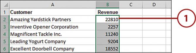
1. Select the range of values to which you want to apply the formatting.
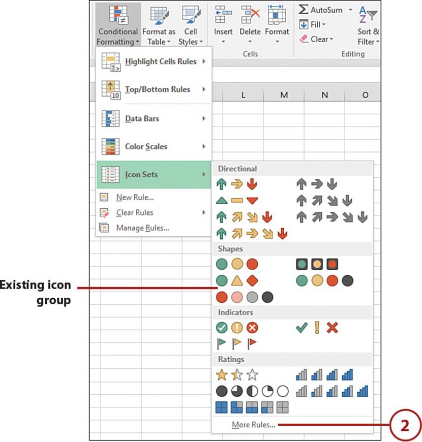
2. Select Icon Sets, More Rules from the Conditional Formatting drop-down on the Home tab.
Use Existing Icon Group
You can choose an icon group from the Icon Style drop-down instead of creating one from scratch. If you do use an existing icon group, then continue to step 6.
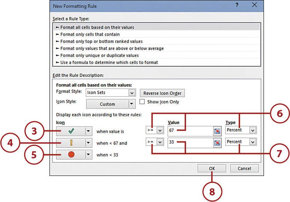
3. Click the first drop-down under the Icon heading and select the green check mark.
4. Click the second drop-down and select the yellow exclamation point.
5. Click the third drop-down and select the red stoplight.
6. To the right of the first drop-down, select >=, enter 67, and select Percent.
7. To the right of the second drop-down, select >=, enter 33, and select Percent.
8. Click OK.
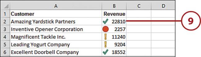
9. The icons will be added to the range. When a value in the range changes, the icon will update accordingly.
Edit Default Icon Sets
Excel has several default icon sets you can quickly apply from the Conditional Formatting drop-down, but you may still need to modify the logic used for each icon. If you select an icon set from the Conditional Formatting drop-down and need to edit the logic values, see the section “Edit Conditional Formatting.”
Highlight the Top 10
You can format the top 10 values in a dataset so they stand out.
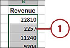
1. Select the range to which you want to apply the formatting. The comparison and formatting will apply to all numerical values selected, even if they are in different columns.
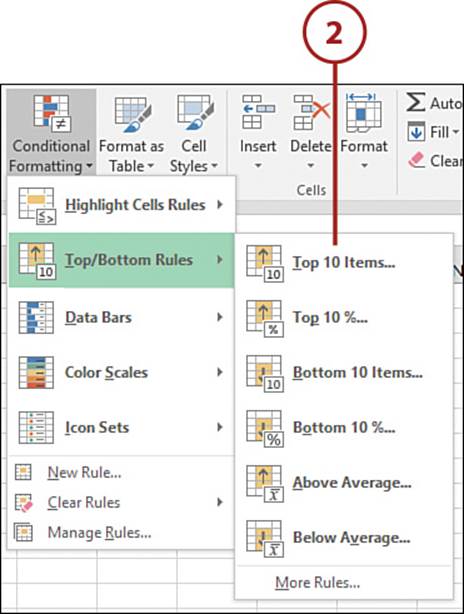
2. Select Top/Bottom Rules, Top 10 Items from the Conditional Formatting drop-down on the Home tab.
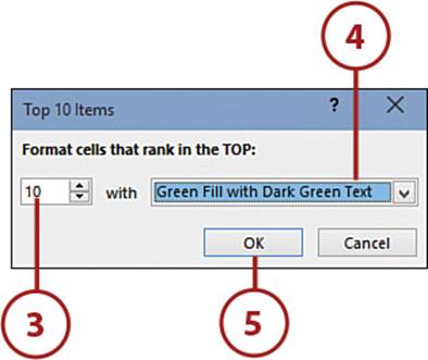
3. Change the value if you want something other than the top 10.
4. Select the desired formatting option. As you choose, your dataset will update so you can see how the formatting looks.
More Formatting Options
If you click Custom Format from the list of formatting options in the dialog box, the Format Cells dialog box will open up and you can use it to create your own format.
5. Click OK.
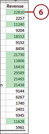
6. The conditional format will be applied to the dataset. As the values change, the formatting will automatically update.
Highlight Entire Row
If you need to highlight the entire row of the dataset, you’ll have to set up a conditional format using a formula rule. See “Create a Custom Rule” for more information.
>>>Go Further: More Predefined Rules
The Conditional Formatting drop-down contains more predefined rules under Highlight Cells Rules and Top/Bottom Rules:
• Cells containing values greater than, less than, between, or equal to the value you specify
• Cells containing specific text
• Cells containing a date from the last day, two days, and so on
• Cells containing duplicate values
• Cells containing the top or bottom n items
• Cells containing the top or bottom n%
• Cells containing values above or below the average
You can apply multiple predefined rules to a single selection—for example, highlight the top 10 and those values that fall within a certain range.
Highlight Duplicate or Unique Values
Use the preset conditional formats to highlight duplicate or unique data in a range.
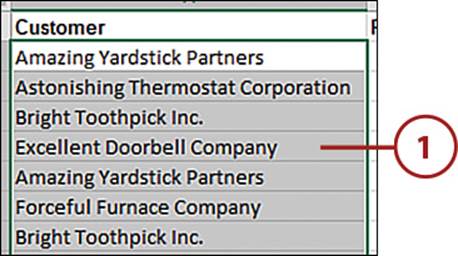
1. Select the range to which you want to apply the formatting.
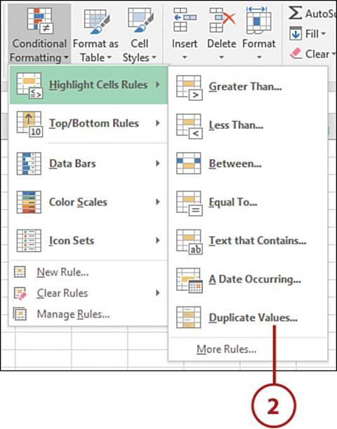
2. Select Highlight Cells Rules, Duplicate Values from the Conditional Formatting drop-down on the Home tab.
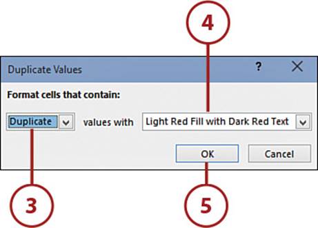
3. Select Duplicate to highlight the duplicate data. Select Unique to highlight the unique data.
4. Select the desired formatting option. As you choose, your dataset will update so you can see how the formatting looks.
5. Click OK.
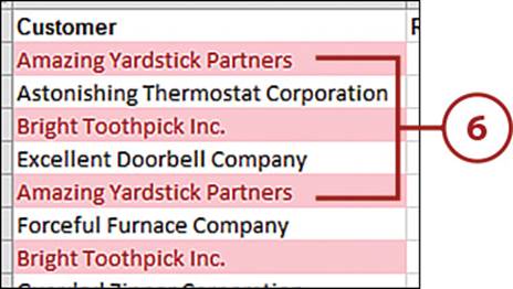
6. The duplicate or unique data will be highlighted.
Create a Custom Rule
You can customize any of the prebuilt rules, but if what you need is not listed, such as highlighting a row based on a selection from a drop-down, you’ll want to build your own conditional formatting rule based on a formula.
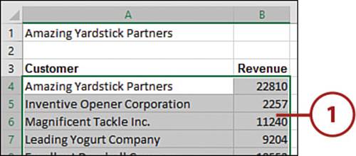
1. Select the range to which you want to apply the formatting, including all the columns you want highlighted.
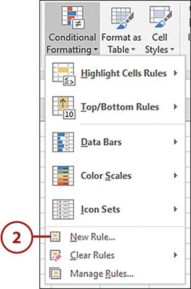
2. Select New Rule from the Conditional Formatting drop-down on the Home tab.
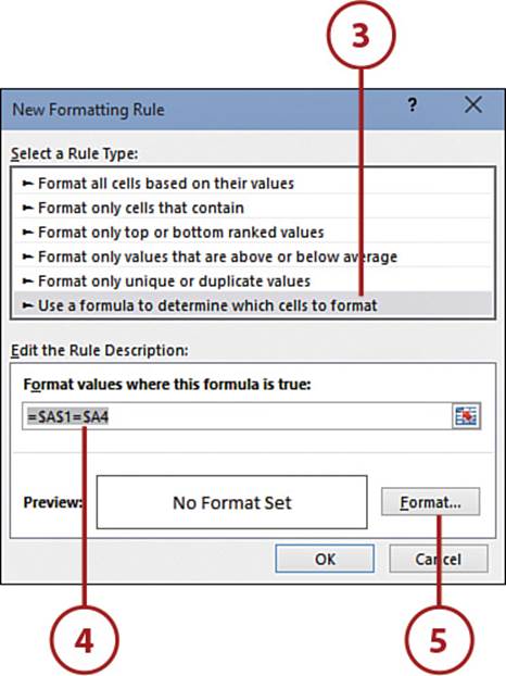
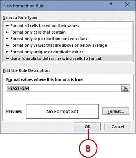
3. Select the Use a Formula to Determine Which Cells to Format option.
4. Enter a logical formula that will evaluate to True or False. For example:
=$A$1=$A4
5. Click the Format button to open the Format Cells dialog box.
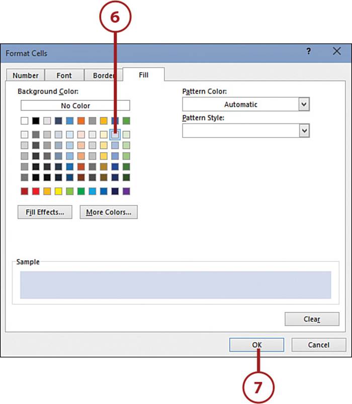
6. Select the desired formatting options (for example, a light blue fill).
7. Click OK when you’re done formatting.
8. Click OK to return to the sheet.
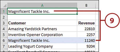
9. When a different name is entered in a cell, for example A1, the corresponding record will be highlighted.
>>>Go Further: Understanding the Formula
Conditional formulas must evaluate to True or False.
In the previous example, $A$1 is the cell with the company name to match. The reference is absolute so that as the value is compared to other cells in the selected range, the address won’t change, similar to copying down a formula. If we need to match values in column B, then the address would be $B$1.
$A4 is the first cell in the selected range that has a possible match. Only the column is absolute so that when the comparison is done to values in column B, the column reference doesn’t change. However, when the comparison is done to another row, the row number does update. For example, the formula in B4 is (if you could see it) $A$1=$A4; the formula in A5 is $A$1=$A5; the formula in B5 is $A$1=$A5.
For more information on absolute versus relative referencing, see Chapter 8, “Using Formulas.”
Clear Conditional Formatting
With a few clicks of the mouse, you can clear all conditional formatting from a selected range.
Delete Specific Rules
If you need to delete specific rules, refer to the section “Edit Conditional Formatting” to learn how to open the dialog box from which you can select and delete rules.
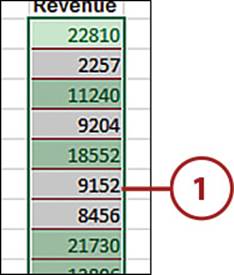
1. Select the range from which you want to clear the conditional formatting.
2. From the Clear Rules submenu in the Conditional Formatting drop-down on the Home tab, select Clear Rules from Selected Cells.
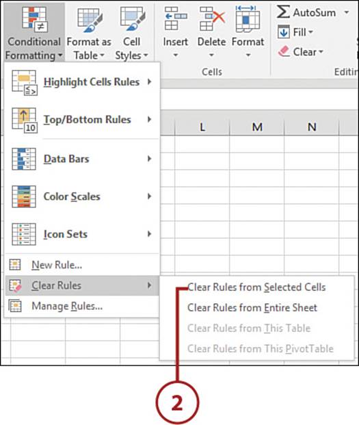
3. The rules will be cleared from the selection. If there are other ranges with one or more of the same rules, the rules will still apply to those ranges. If there are no other ranges, the rules will be deleted.
Edit Conditional Formatting
You can edit conditional formatting to change the rule itself, the range to which it is applied, or both.
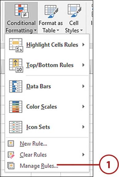
1. Select Manage Rules from the Conditional Formatting drop-down on the Home tab.
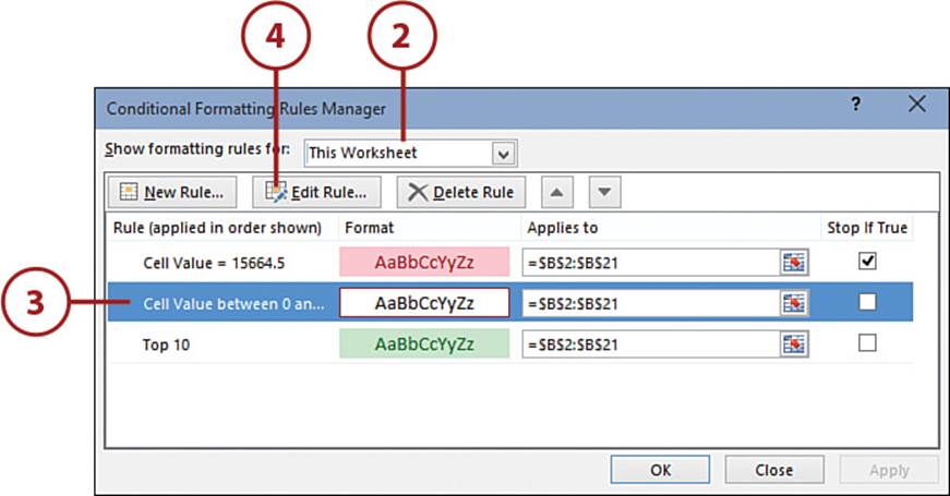
2. Choose which rules you want to view. For example, choose This Worksheet to view all the rules on the sheet.
3. Highlight the rule you want to edit.
4. Click Edit Rule.
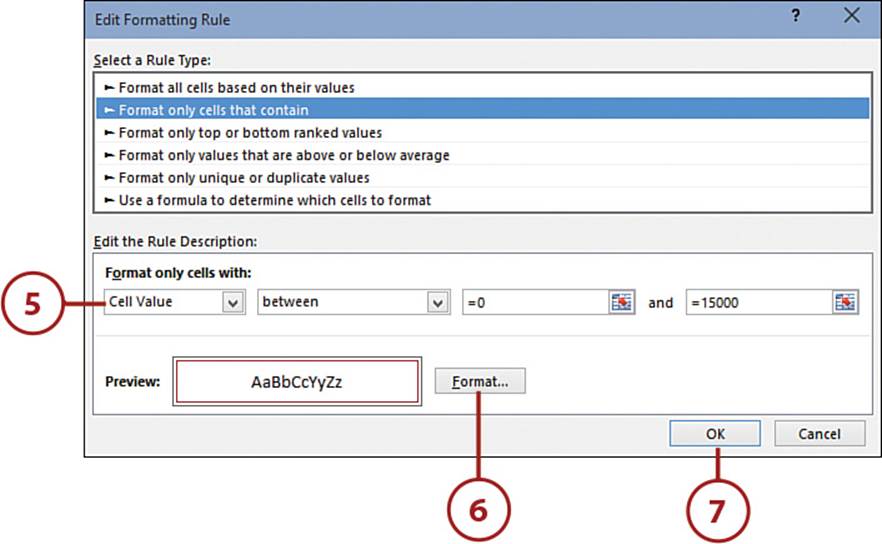
5. Make the desired changes to the rule.
6. Click Format to change the formatting used.
7. Click OK.
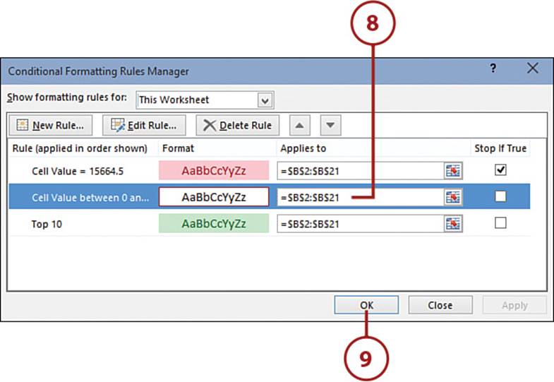
8. To change the range to which the rule is applied, click in the address field and then select a new range on the sheet. You can also type the address directly in the field, but ensure the cell addresses are absolute.
9. Click OK to apply the changes.
Using Cell Styles to Apply Cell Formatting
You’re probably familiar with using styles in Word but never realized that styles are also available in Excel. Styles provide a great way of quickly applying consistent formatting in your workbooks.
Apply a Style
As you move your pointer over the styles, the selected range will update, providing a preview of the style on the sheet.
1. Select the range to which you want to apply the style.

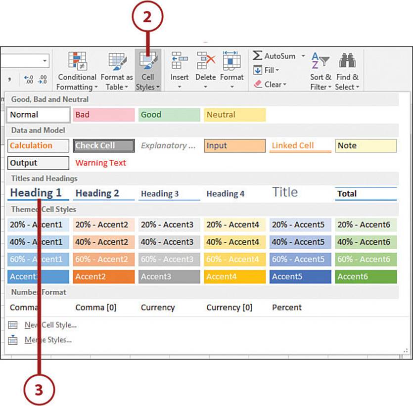
2. On the Home tab, click the Cell Styles drop-down to view the styles.
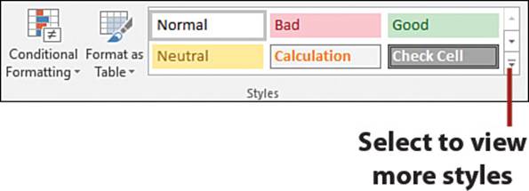
No Cell Styles Button Visible
If your monitor is large enough and resolution set high, you won’t see the Cell Styles button—you’ll see a selection of styles directly on the ribbon. Click the drop-down in the bottom-right corner to view more styles.
3. Select the desired style, such as Heading 1.
4. The selected range will update to the new style.

Style a Table
If your dataset is setup as a table (when you select a cell in the dataset, you see the Table Tools ribbon tab), you have the additional option of using the Table Styles on the Table Tools, Design tab. Note that Cell Styles will overwrite Table Styles.
Create a Custom Style
You aren’t limited to these predefined styles. You can create and save your own style for use throughout the workbook it’s saved in.
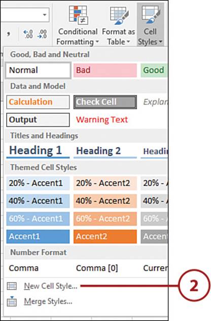
1. Apply the desired formatting to a cell. You can also start from a preexisting style and make changes to it. Select the cell.

2. On the Home tab, select New Cell Style from the Cell Styles drop-down.
3. Enter a new style name.
4. Select the options you want included in the style.
5. Click OK.
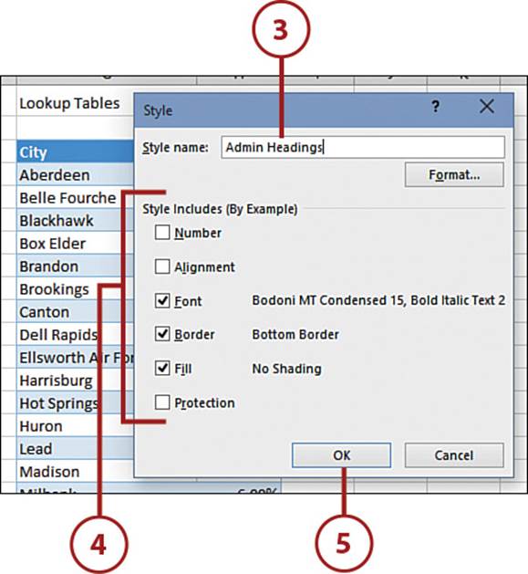
6. The custom style will appear at the top of the style drop-down. See the section “Apply a Style” for instruction on how to apply the style.
Using Themes to Ensure Uniformity in Design
Themes are collections of fonts, colors, and graphic effects that can be applied to a workbook. This can be useful if you have a series of company reports that need to have the same color and fonts. Only one theme can affect a workbook at a time.
Excel includes several built-in themes, which you can access from the Themes drop-down on the Page Layout tab. You can also create and share themes you design.
A theme has the following elements, which you can apply individually instead of applying an entire theme package:
• Fonts—A theme includes a font for headings and a font for body text.
• Colors—There are 12 colors in a theme: four for text, six for accents, and two for hyperlinks.
• Graphic effects—Graphic effects include lines, fills, bevels, shadows, and so on.
Apply a New Theme
Excel has a variety of themes you can choose from.
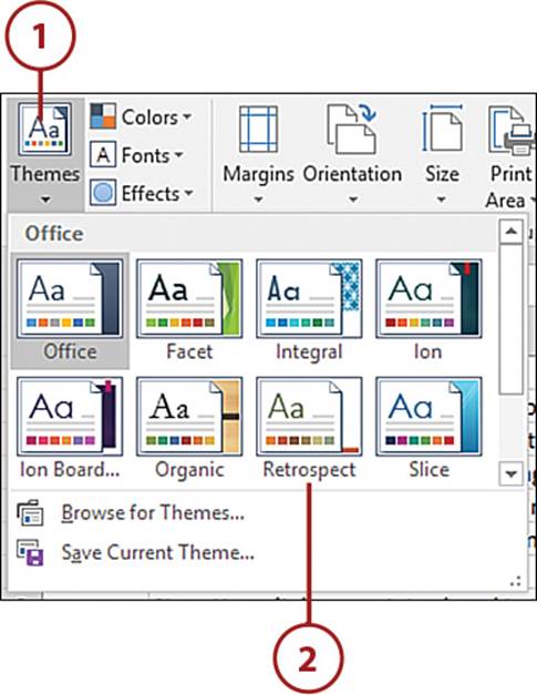
1. On the Page Layout tab, open the Themes drop-down.
2. As you move the pointer over a theme, the objects (fonts, charts, and so on) on the active sheet will change to reflect that theme. When you find one you like, click it, and it will be applied to the workbook.
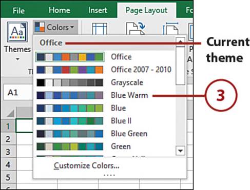
3. If you like some elements of a theme, but not others, open the drop-down corresponding to the element you want to change (Colors, Fonts, or Effects) and select a new palette.
Create a New Theme
When you create and save a theme, you can apply it to other workbooks or share it with other people. First change the colors, fonts, and/or effects as desired and then save that combination as a new theme.
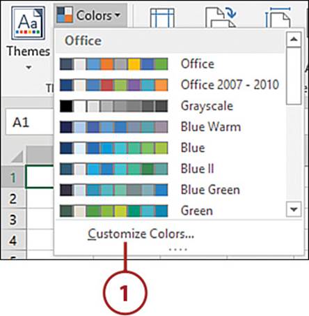
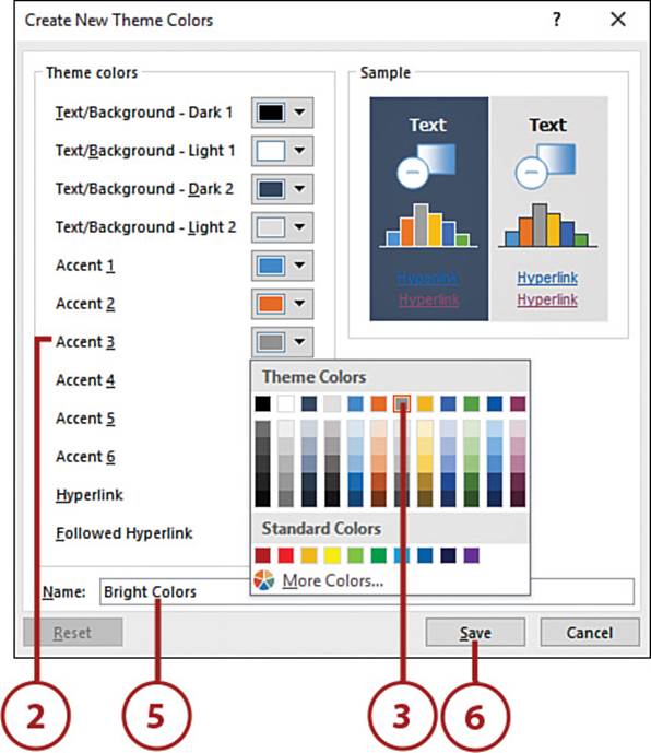
1. Select Customize Colors from the Colors drop-down on the Page Layout tab.
2. To change the color for one of the color placeholders, such as Accent 3, choose its drop-down to open the color palette.
3. When you find the desired color, click it to apply it to your theme.
4. Repeat steps 2 and 3 for each color placeholder you want to change.
5. Type a name for your color theme.
6. Click Save.
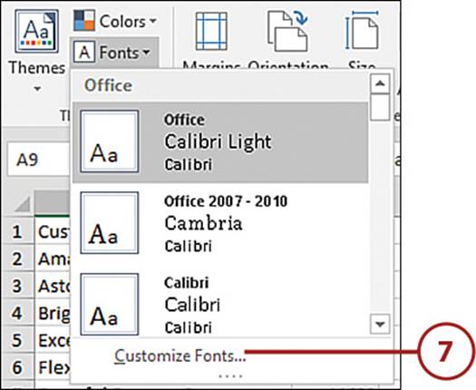
7. Select Customize Fonts from the Fonts drop-down on the Page Layout tab.
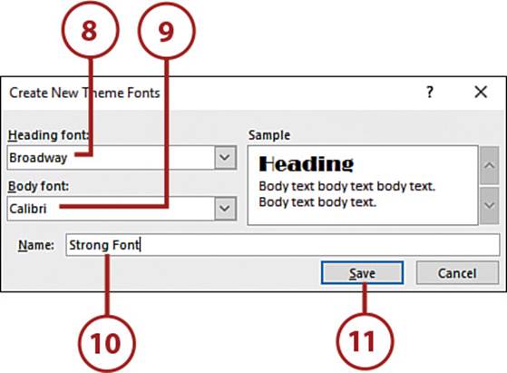
8. Click the Heading Font drop-down and choose a new font.
9. Click the Body Font drop-down and choose a new font.
10. Type a name for your font theme.
11. Click Save.
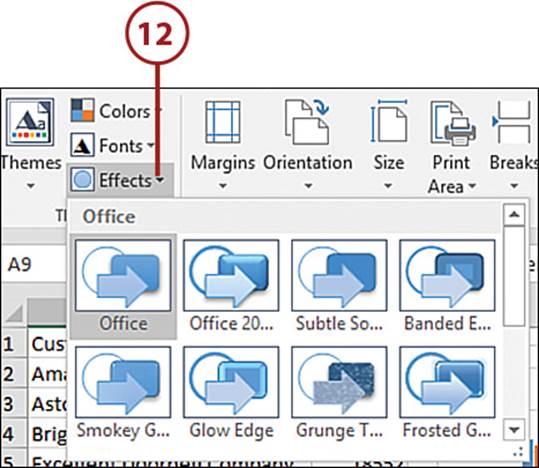
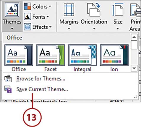
12. Select an effect from the gallery of built-in effects from the Effects drop-down on the Page Layout tab.
13. Select Save Current Theme from the Themes drop-down on the Page Layout tab.
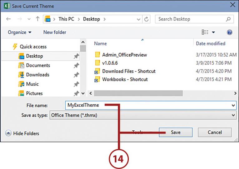
14. Browse to a location to save the theme and enter a name for it. Click Save.
Share a Theme
To share a theme with other people, you must send them the *.thmx file you saved when you created the theme (refer to “Create a New Theme”).
When the other people receive the file, they should save it to either their equivalent theme folder or some other location and then use the Browse for Themes option under Themes on the Page Layout tab.
All materials on the site are licensed Creative Commons Attribution-Sharealike 3.0 Unported CC BY-SA 3.0 & GNU Free Documentation License (GFDL)
If you are the copyright holder of any material contained on our site and intend to remove it, please contact our site administrator for approval.
© 2016-2026 All site design rights belong to S.Y.A.