Microsoft Office 2016 At Work For Dummies (2016)
Chapter 10
Storing and Managing Databases in Excel
In This Chapter
![]() Entering database data in Excel
Entering database data in Excel
![]() Converting between a range and a table
Converting between a range and a table
![]() Sorting a table
Sorting a table
![]() Filtering a table
Filtering a table
![]() Referring to named ranges in formulas in a table
Referring to named ranges in formulas in a table
![]() Creating and saving a query
Creating and saving a query
![]() Removing duplicates from a dataset
Removing duplicates from a dataset
![]() Validating data to minimize entry errors
Validating data to minimize entry errors
Besides its calculation capabilities, Excel also has some great features for managing databases. You can store, search, sort, and filter large lists of information with ease in Excel. And by converting a range to a table in Excel, you can access certain sorting and filtering commands even more easily.
In this chapter, you learn some database concepts and find out how to create and manage tables in a workbook. You’ll also learn how to create and save a query, remove duplicates from a dataset, and use data validation to minimize data entry errors.
Create an Excel database
Here are a few terms you need to know. A database is a collection of information stored in a consistent, structured way. An address book is a database, for example, because it stores the same pieces of information about each person: name, address, city, state, and ZIP code. In that example, each type of information is a field. Each person’s complete entry (all fields) is a record. The collection of data as a whole is called a table, or dataset.
In a database table in Excel:
![]() Each column is a field. The field names appear in the first row.
Each column is a field. The field names appear in the first row.
![]() Each record appears in a separate row beneath the column headings.
Each record appears in a separate row beneath the column headings.
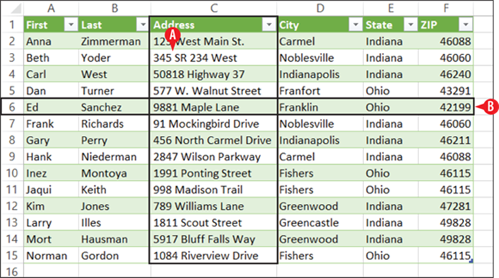
Figure 10-1: A simple database in an Excel table.
Tables have several advantages over ranges:
· You can filter by columns using an easy drop-down list.
· You can add a Totals row that adds summary calculations without having to manually enter the formula for it.
· You can apply table formatting presets.
· You can publish a table to a SharePoint server.
Convert a range to a table
Before you convert a range to a table, make sure you have properly prepared the range. Specifically, you need to do the following:
· Make sure that the first row contains the field names you want to use. The entries in the first row will become column headings.
· Make sure that each row contains one and only one record.
· Make sure that there are no blank rows between rows containing records
When the data is cleaned up and ready to go, follow these steps:
![]() Select the range of data that should become a table.
Select the range of data that should become a table.
![]() On the Insert tab, click Table. The Create Table dialog box opens.
On the Insert tab, click Table. The Create Table dialog box opens.
![]() Confirm that the range is correct.
Confirm that the range is correct.
![]() Click OK. The range is converted to a table and the default table formatting style is applied to it.
Click OK. The range is converted to a table and the default table formatting style is applied to it.
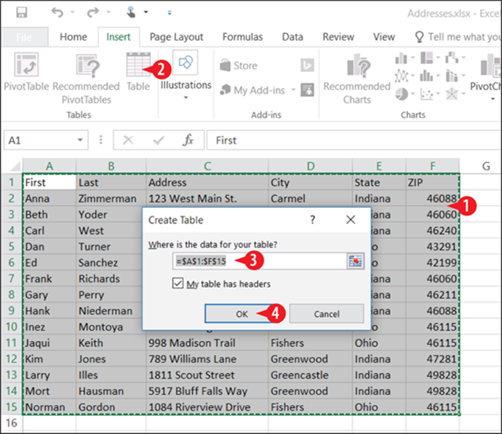
Figure 10-2: Convert a range to a table using the Insert tab’s Table command.
Convert a range to a table and choose a table style
Here’s an alternate method that enables you to specify the table formatting style you want:
![]() Select the range of data that should become a table.
Select the range of data that should become a table.
![]() On the Home tab, click Format as Table.
On the Home tab, click Format as Table.
![]() Click the desired format. The Format as Table dialog box opens. (It’s exactly the same as the Create Table dialog box shown in Figure 10-2 except for its name.)
Click the desired format. The Format as Table dialog box opens. (It’s exactly the same as the Create Table dialog box shown in Figure 10-2 except for its name.)
4. Confirm that the range is correct.
5. Click OK. The range is converted to a table and the chosen table formatting style is applied to it.
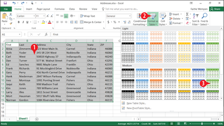
Figure 10-3: Convert a range to a table by applying table formatting to it.
Change the table appearance
After a range has been converted to a table, you can modify its appearance by adjusting the table style.
To choose a different table style, on the Table Tools Design tab, choose a different style from the Table Styles gallery. (See ![]() in Figure 10-4.)
in Figure 10-4.)
Fine-tune the table’s appearance by marking or clearing check boxes in the Table Style Options group:
![]() Header Row turns the display of the header row on/off.
Header Row turns the display of the header row on/off.
![]() Total Row toggles a total row at the bottom of the table. In tables with numeric data that can be summarized, this is great, but in a database that is purely unrelated records, like in an address book, it makes no sense to use this.
Total Row toggles a total row at the bottom of the table. In tables with numeric data that can be summarized, this is great, but in a database that is purely unrelated records, like in an address book, it makes no sense to use this.
![]() Banded Rows and Banded Columns toggle the use of shading in alternate rows or columns to make the data easier to browse.
Banded Rows and Banded Columns toggle the use of shading in alternate rows or columns to make the data easier to browse.
![]() First Column and Last Column make their respective columns formatted differently from the others in the table; this is useful if those columns contain headings or summary data.
First Column and Last Column make their respective columns formatted differently from the others in the table; this is useful if those columns contain headings or summary data.
![]() Filter Button toggles the down-pointing arrow button on each field name at the top of the table.
Filter Button toggles the down-pointing arrow button on each field name at the top of the table.
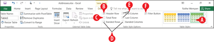
Figure 10-4: Control table formatting on the Table Tools Design tab.
Convert a table to a range
If you decide you want the dataset to go back to being a regular range, you can easily restore that status. Here’s how:
![]() Select any cell within the table.
Select any cell within the table.
![]() On the Table Tools Design tab, click Convert to Range.
On the Table Tools Design tab, click Convert to Range.
![]() Click Yes to confirm. The range is no longer a table; however, it retains any formatting that it had as a table.
Click Yes to confirm. The range is no longer a table; however, it retains any formatting that it had as a table.
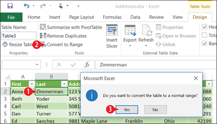
Figure 10-5: Convert a table back to a range.
 If you want to remove the table formatting, select the range and choose Home ⇒ Clear ⇒ Clear Formats.
Sort a table
You can sort a table’s data by a single field or by multiple fields.
Sort by a single field
When you sort by a single field, Excel rearranges the records in A to Z (ascending) or Z to A (descending) order based on the field you specify.
There are several ways to sort by a single field, including the following:
![]() Click any cell in the desired column and then click the AZ or ZA button on the Data tab.
Click any cell in the desired column and then click the AZ or ZA button on the Data tab.
![]() Right-click any cell in the desired column, point to Sort, and then click Sort A to Z or Sort Z to A. (The wording of the choices is different if the column contains numbers or dates.)
Right-click any cell in the desired column, point to Sort, and then click Sort A to Z or Sort Z to A. (The wording of the choices is different if the column contains numbers or dates.)
![]() Click the arrow at the top of the column to open its menu, and then click Sort A to Z or Sort Z to A. (Again, the wording of the choices is different if the column contains numbers or dates.)
Click the arrow at the top of the column to open its menu, and then click Sort A to Z or Sort Z to A. (Again, the wording of the choices is different if the column contains numbers or dates.)
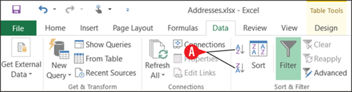
Figure 10-6: Use the Sort Ascending (AZ) or Sort Descending (ZA) button for a quick one-column sort.
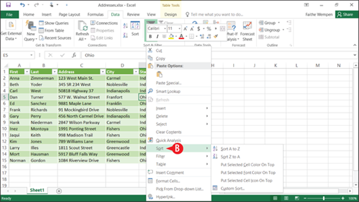
Figure 10-7: Right-click in the column, choose Sort, and click the desired sort.
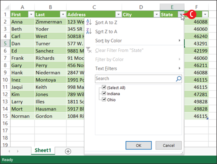
Figure 10-8: Open the column’s menu and choose a sort option.
Sort by multiple fields
When you sort by multiple fields, it does a single sort by the first field you specify, and then in the event of a tie for that field, it relies on the additional field(s) you specify to break the tie. For example, if you sort first by City and then by State, Decatur GA will come before Decatur IL.
To sort by multiple fields:
![]() Click anywhere within the table to sort. It does not have to be within a specific column.
Click anywhere within the table to sort. It does not have to be within a specific column.
![]() On the Data tab, click Sort. The Sort dialog box opens.
On the Data tab, click Sort. The Sort dialog box opens.
![]() Open the Sort by drop-down list and choose the first field on which to sort.
Open the Sort by drop-down list and choose the first field on which to sort.
![]() Open the Order drop-down list and choose the desired order.
Open the Order drop-down list and choose the desired order.
![]() Click Add Level.
Click Add Level.
6. For the newly added level, repeat steps 3-4.
![]() Add more levels if needed; click OK when finished.
Add more levels if needed; click OK when finished.
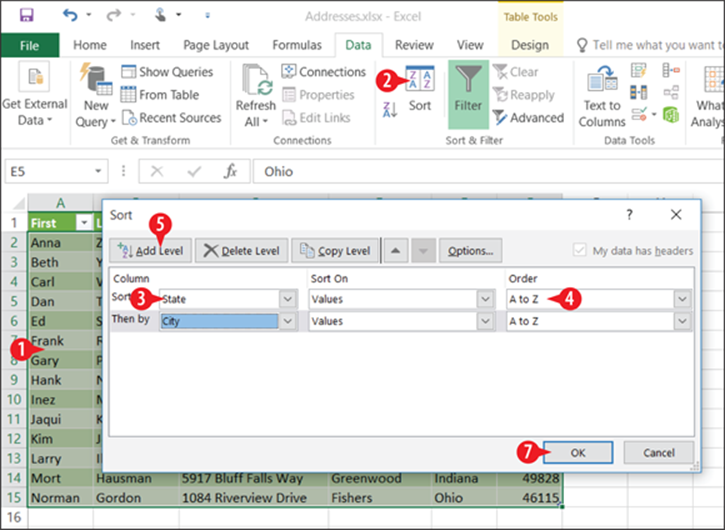
Figure 10-9: Choose multiple sort fields and the order in which they will be applied.
Remove a sort or filter
When a table has been sorted, the button at the top of the column shows an up-pointing or down-pointing arrow on it, depending on whether you sorted in ascending or descending order. (See ![]() in Figure 10-10.)
in Figure 10-10.)
To clear the sort (and also clear any filters that have been applied):
![]() Click any cell in the table.
Click any cell in the table.
![]() Click the Clear button on the Data tab.
Click the Clear button on the Data tab.
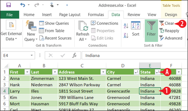
Figure 10-10: Sorted data columns appear with an extra arrow on their button.
Filter a table
Filtering data means to hide certain records, displaying only the ones that match criteria you specify. There are several ways to specify filter criteria.
Filter by selection
Perhaps the easiest filtering technique is to filter by selection, which hides all records where the specified field does not contain a sample value you select. Here’s how to do it:
![]() Click a cell in the table that contains the value by which you want to filter. For example, to show only addresses with Indianapolis as the city, select a cell in the City column that contains Indianapolis.
Click a cell in the table that contains the value by which you want to filter. For example, to show only addresses with Indianapolis as the city, select a cell in the City column that contains Indianapolis.
![]() Right-click the cell, and then point to Filter.
Right-click the cell, and then point to Filter.
![]() Click Filter by Selected Cell’s Value.
Click Filter by Selected Cell’s Value.
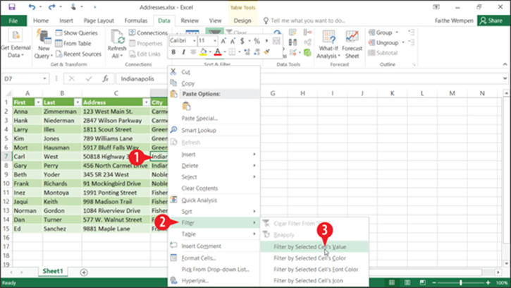
Figure 10-11: Filter by one specific value in one field.
A filter is immediately applied so that only records that match that value in that field are shown.
Filter by choosing values from a list
If you want to filter by more than one value in a field, here’s a technique that enables you to do so:
![]() Click the arrow on the column containing the values by which you want to filter.
Click the arrow on the column containing the values by which you want to filter.
![]() Clear the check boxes for each value that you do not want to include.
Clear the check boxes for each value that you do not want to include.
In step 2, if you want only a few values to be selected, click the (Select All) check box to clear all check boxes, and then mark just the few you want.
![]() Click OK. The filter is applied.
Click OK. The filter is applied.
4. (Optional) To filter the data even further, repeat steps 1-4 for additional columns.
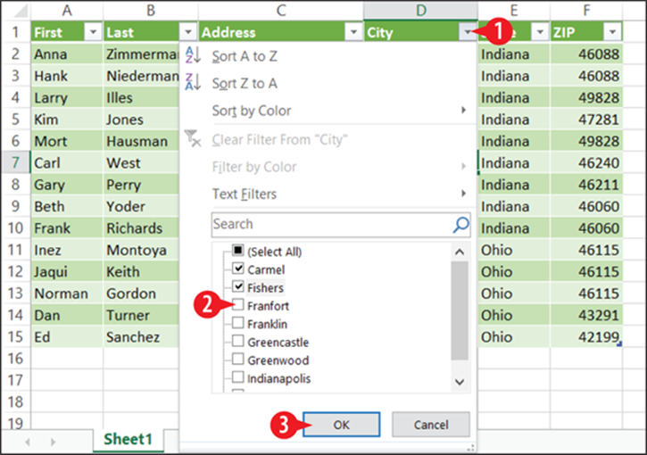
Figure 10-12: Filter by choosing which values to include or exclude.
Filter using conditions
Depending on the content of the field (text, date, number, etc.) you can also use conditions for that type of data, such as Begins With, Ends With, or Contains (for text) or Greater Than, Less Than, or Between (for numbers).
For a field that contains text, do the following:
![]() Click the arrow on the column containing the values by which you want to filter.
Click the arrow on the column containing the values by which you want to filter.
![]() Point to Text Filters (if it’s a text field) or the equivalent command for number or date field if appropriate.
Point to Text Filters (if it’s a text field) or the equivalent command for number or date field if appropriate.
![]() Click the desired logical condition, such as Begins With.
Click the desired logical condition, such as Begins With.
![]() In the Custom AutoFilter dialog box, specify the condition value. You can optionally enter a second condition, too.
In the Custom AutoFilter dialog box, specify the condition value. You can optionally enter a second condition, too.
Use ? to represent a single character or * to represent any number of characters.
![]() Click OK. The filter is applied.
Click OK. The filter is applied.
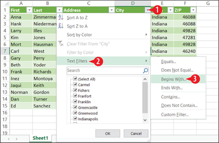
Figure 10-13: Choose a condition.
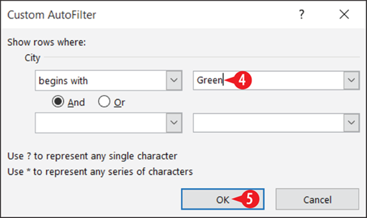
Figure 10-14: Define the condition(s).
Add a Total row to a table
One of the advantages of making a data range into a table is the ability to show a Total row as part of the table, summarizing one or more columns that you specify. Contrary to its name, a total row can do more than just total (add). A total row performs a summary operation of your choice on any field(s) in the table. For example, you can average, count, sum, or find the minimum, maximum, or standard deviation of that column’s data.
![]() To enable the total row, on the Table Tools Design tab, mark the Total Row check box.
To enable the total row, on the Table Tools Design tab, mark the Total Row check box.
The Total row appears at the bottom of the table. Each of the cells in that row now have their own arrow that opens a menu.
![]() At the bottom of a column that contains data you want to summarize, click the arrow to open the drop-down list.
At the bottom of a column that contains data you want to summarize, click the arrow to open the drop-down list.
The arrow for a cell appears just outside the cell to its right.
There are more options available when working with a numeric field, but even text fields have some totals they can display, such as a count of the number of records. You can use any function in Excel for this, but the most common ones are available from a menu for easy access.
If a column has a calculation in the Total row that you don’t want, click the arrow on that cell to open its menu and choose None. (See ![]() in Figure 10-16.)
in Figure 10-16.)
![]() Click the kind of calculation you want.
Click the kind of calculation you want.
![]() (Optional) Type a text label in an adjacent cell to describe the calculation you chose.
(Optional) Type a text label in an adjacent cell to describe the calculation you chose.
If you want a function that isn’t on the list in Figure 10-16, choose More Functions, and then choose from the Insert Function dialog box, just as you would if you used the Insert Function command on the Formulas tab in a normal range. (See ![]() in Figure 10-16.)
in Figure 10-16.)
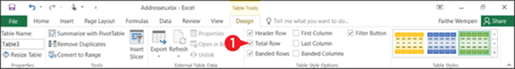
Figure 10-15: Enable the total row by marking the Total Row check box.
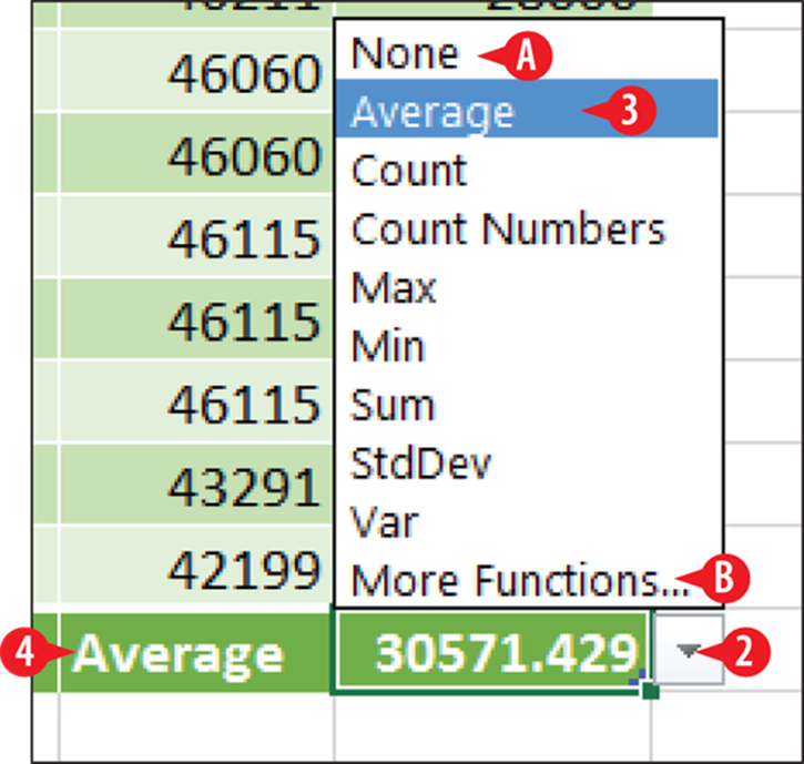
Figure 10-16: Select the desired calculation. Use text labels to make sure your meaning is clear.
Create queries
When you sort and filter a table in a certain way, it may take you a few minutes to set up those conditions. Wouldn’t it be nice to be able to save that sorting and filtering specification to use again later? A query does that and can also do much more. For example, a query can also temporarily hide certain columns as well as sort and filter rows.
Although the full query capabilities of Excel are beyond the scope of this book, the following steps give you a little taste of it.
To create a query:
![]() Click anywhere within the table.
Click anywhere within the table.
![]() On the Data tab, click From Table. A Query Editor window opens.
On the Data tab, click From Table. A Query Editor window opens.
![]() Sort the data the way you want it. Use the AZ and ZA buttons on the Home tab or open a column’s menu and choose a sort order for that column.
Sort the data the way you want it. Use the AZ and ZA buttons on the Home tab or open a column’s menu and choose a sort order for that column.
![]() Filter the data to include only the records you want. Use a column’s menu to set up the filter, as you learned earlier in this chapter.
Filter the data to include only the records you want. Use a column’s menu to set up the filter, as you learned earlier in this chapter.
If you want to remove one of the instructions, click it in the Applied Steps box and then click the X to its left. (See ![]() in Figure 10-18.)
in Figure 10-18.)
![]() If you want to exclude certain columns, click Choose Columns. Clear the check box for each column to exclude and click OK.
If you want to exclude certain columns, click Choose Columns. Clear the check box for each column to exclude and click OK.
![]() Change the name in the Name box to something meaningful for the instructions you specified.
Change the name in the Name box to something meaningful for the instructions you specified.
![]() Click Close & Load. The query results appear on a new sheet in the workbook.
Click Close & Load. The query results appear on a new sheet in the workbook.
The query results sheet becomes a permanent part of your workbook. Any time you want to view the query results, just display that worksheet. However, the data on the query results sheet doesn’t automatically update when the data changes on the original sheet. Therefore you will want to refresh the query whenever the original data changes. To do this, on the Data tab, click Refresh All. (See ![]() in Figure 10-19.)
in Figure 10-19.)
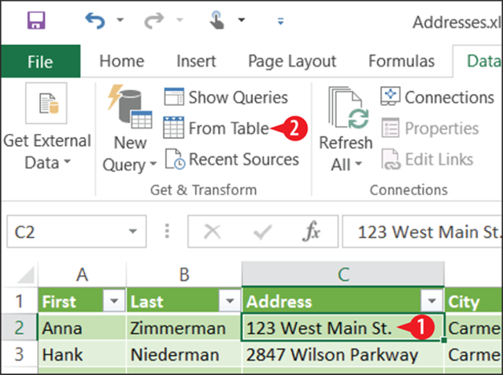
Figure 10-17: Start a new query based on a table.
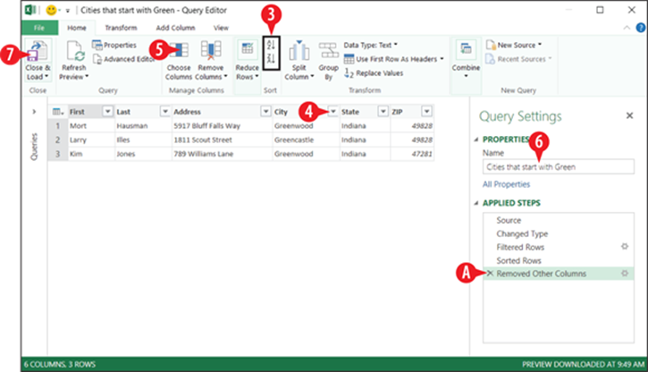
Figure 10-18: Define the query specification.
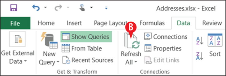
Figure 10-19: Click Refresh All to refresh all results.
Remove duplicates from a dataset
A dataset may contain records for which certain fields are identical, and usually that is not a problem. For example, you might have multiple people with the same last name, address, and phone number if they all live in the same household.
In some cases, though, duplicate values in multiple fields may signal that the same record has been accidentally entered multiple times. For example, if two people both have the same Social Security number, that’s probably an entry error.
You can define a Remove Duplicates operation so that multiple fields must all be identical in order for a deletion to occur. For example, you might delete records with the same phone number only if both the first name and last name are identical.
 When removing duplicates, you don’t get to select which of the duplicates will be deleted; the first instance is kept and all others are deleted. Therefore if it’s important that the most recently entered record be kept, sort the table in descending order by a Date field first.
To find duplicates:
![]() Click anywhere in the table.
Click anywhere in the table.
![]() On the Data tab, click Remove Duplicates.
On the Data tab, click Remove Duplicates.
![]() Mark or clear check boxes as needed to define which fields must all be duplicate in order for records to qualify for deletion.
Mark or clear check boxes as needed to define which fields must all be duplicate in order for records to qualify for deletion.
![]() Click OK.
Click OK.
5. At the confirmation box, click OK.
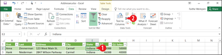
Figure 10-20: Click Remove Duplicates.
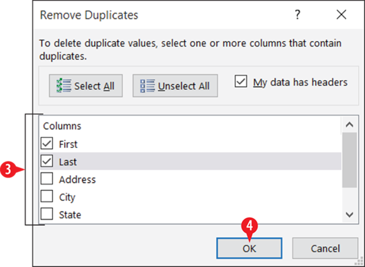
Figure 10-21: Choose which fields to check for duplication.
If the deletion results are not what you expected—for example, if some records were deleted that you meant to keep—use Undo (Ctrl+Z) immediately after the deletion to get them back.
Restrict data entry with validation rules
Data entry errors can cause big headaches in database management. When two entries vary, is it because they are truly different, or did someone just make a mistake? It’s hard to know.
Data entry inconsistencies can also plague a database, especially if multiple people are entering records. For example, should states be entered with their full names or as two-character abbreviations? If the data isn’t consistent, you won’t get accurate results when you query, sort, or filter on a certain state.
A validation rule can limit entry to only certain types of values, such as only integers or dates. It can also limit text entry to a certain number of characters.
Create a validation rule
To create a data validation rule:
![]() Select the cells for which the rule will apply. For example, to restrict entries in a certain field in a table, select that field’s column.
Select the cells for which the rule will apply. For example, to restrict entries in a certain field in a table, select that field’s column.
![]() On the Data tab, click Data Validation.
On the Data tab, click Data Validation.
3. On the Settings tab, open the Allow drop-down list and choose a restriction. Then enter any parameters for that restriction.
For example, if you wanted states to be entered as two-character codes, you might choose Text length and then enter 2 as both the minimum and maximum length, as in Figure 10-23. (See ![]() in Figure 10-23.)
in Figure 10-23.)
Or, if you choose a certain type of entry, such as Whole Number, you can enter a range of whole numbers into which the value must fall, as in Figure 10-24. (See ![]() in Figure 10-24.)
in Figure 10-24.)
![]() Click the Error Alert tab.
Click the Error Alert tab.
![]() In the Title box, enter text to appear in the title bar of an error message box that will appear if the rule is violated.
In the Title box, enter text to appear in the title bar of an error message box that will appear if the rule is violated.
![]() In the Error message box, enter text to appear as the body of the error message.
In the Error message box, enter text to appear as the body of the error message.
![]() Click OK.
Click OK.
When someone violates the rule, the error box appears that you set up in steps 4-6. (See ![]() in Figure 10-26.)
in Figure 10-26.)
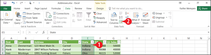
Figure 10-22: Click the Data Validation button.
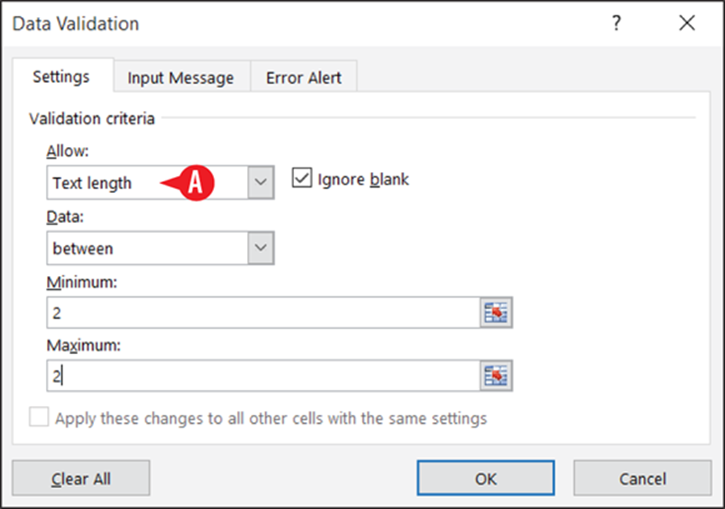
Figure 10-23: A text length validation rule.
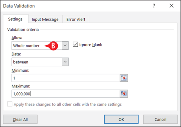
Figure 10-24: An integer validation rule where the number is positive.
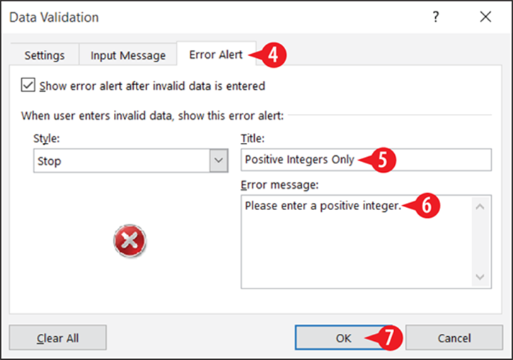
Figure 10-25: Create the error dialog box text.
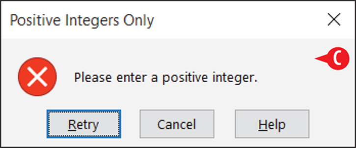
Figure 10-26: The error message appears in a dialog box when the validation rule is broken.
Remove a validation rule
To remove data validation, follow these steps:
1. Select the cell(s) from which to remove data validation.
2. On the Data tab, click Data Validation.
![]() Click Clear All.
Click Clear All.
![]() Click OK.
Click OK.
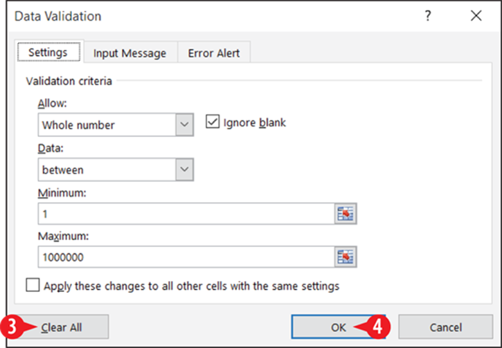
Figure 10-27: Clear data validation rules from the selected cell(s).
All materials on the site are licensed Creative Commons Attribution-Sharealike 3.0 Unported CC BY-SA 3.0 & GNU Free Documentation License (GFDL)
If you are the copyright holder of any material contained on our site and intend to remove it, please contact our site administrator for approval.
© 2016-2026 All site design rights belong to S.Y.A.