Hadoop: The Definitive Guide (2015)
Part IV. Related Projects
Chapter 19. Spark
Apache Spark is a cluster computing framework for large-scale data processing. Unlike most of the other processing frameworks discussed in this book, Spark does not use MapReduce as an execution engine; instead, it uses its own distributed runtime for executing work on a cluster. However, Spark has many parallels with MapReduce, in terms of both API and runtime, as we will see in this chapter. Spark is closely integrated with Hadoop: it can run on YARN and works with Hadoop file formats and storage backends like HDFS.
Spark is best known for its ability to keep large working datasets in memory between jobs. This capability allows Spark to outperform the equivalent MapReduce workflow (by an order of magnitude or more in some cases[128]), where datasets are always loaded from disk. Two styles of application that benefit greatly from Spark’s processing model are iterative algorithms (where a function is applied to a dataset repeatedly until an exit condition is met) and interactive analysis (where a user issues a series of ad hoc exploratory queries on a dataset).
Even if you don’t need in-memory caching, Spark is very attractive for a couple of other reasons: its DAG engine and its user experience. Unlike MapReduce, Spark’s DAG engine can process arbitrary pipelines of operators and translate them into a single job for the user.
Spark’s user experience is also second to none, with a rich set of APIs for performing many common data processing tasks, such as joins. At the time of writing, Spark provides APIs in three languages: Scala, Java, and Python. We’ll use the Scala API for most of the examples in this chapter, but they should be easy to translate to the other languages. Spark also comes with a REPL (read — eval — print loop) for both Scala and Python, which makes it quick and easy to explore datasets.
Spark is proving to be a good platform on which to build analytics tools, too, and to this end the Apache Spark project includes modules for machine learning (MLlib), graph processing (GraphX), stream processing (Spark Streaming), and SQL (Spark SQL). These modules are not covered in this chapter; the interested reader should refer to the Apache Spark website.
Installing Spark
Download a stable release of the Spark binary distribution from the downloads page (choose the one that matches the Hadoop distribution you are using), and unpack the tarball in a suitable location:
% tar xzf spark-x.y.z-bin-distro.tgz
It’s convenient to put the Spark binaries on your path as follows:
% export SPARK_HOME=~/sw/spark-x.y.z-bin-distro
% export PATH=$PATH:$SPARK_HOME/bin
We’re now ready to run an example in Spark.
An Example
To introduce Spark, let’s run an interactive session using spark-shell, which is a Scala REPL with a few Spark additions. Start up the shell with the following:
% spark-shell
Spark context available as sc.
scala>
From the console output, we can see that the shell has created a Scala variable, sc, to store the SparkContext instance. This is our entry point to Spark, and allows us to load a text file as follows:
scala> val lines = sc.textFile("input/ncdc/micro-tab/sample.txt")
lines: org.apache.spark.rdd.RDD[String] = MappedRDD[1] at textFile at
<console>:12
The lines variable is a reference to a Resilient Distributed Dataset, abbreviated to RDD, which is the central abstraction in Spark: a read-only collection of objects that is partitioned across multiple machines in a cluster. In a typical Spark program, one or more RDDs are loaded as input and through a series of transformations are turned into a set of target RDDs, which have an action performed on them (such as computing a result or writing them to persistent storage). The term “resilient” in “Resilient Distributed Dataset” refers to the fact that Spark can automatically reconstruct a lost partition by recomputing it from the RDDs that it was computed from.
NOTE
Loading an RDD or performing a transformation on one does not trigger any data processing; it merely creates a plan for performing a computation. The computation is only triggered when an action (like foreach()) is performed on an RDD.
Let’s continue with the program. The first transformation we want to perform is to split the lines into fields:
scala> val records = lines.map(_.split("\t"))
records: org.apache.spark.rdd.RDD[Array[String]] = MappedRDD[2] at map at
<console>:14
This uses the map() method on RDD to apply a function to every element in the RDD. In this case, we split each line (a String) into a Scala Array of Strings.
Next, we apply a filter to remove any bad records:
scala> val filtered = records.filter(rec => (rec(1) != "9999"
&& rec(2).matches("[01459]")))
filtered: org.apache.spark.rdd.RDD[Array[String]] = FilteredRDD[3] at filter at
<console>:16
The filter() method on RDD takes a predicate, a function that returns a Boolean. This one tests for records that don’t have a missing temperature (indicated by 9999) or a bad quality reading.
To find the maximum temperatures for each year, we need to perform a grouping operation on the year field so we can process all the temperature values for each year. Spark provides a reduceByKey() method to do this, but it needs an RDD of key-value pairs, represented by a ScalaTuple2. So, first we need to transform our RDD into the correct form using another map:
scala> val tuples = filtered.map(rec => (rec(0).toInt, rec(1).toInt))
tuples: org.apache.spark.rdd.RDD[(Int, Int)] = MappedRDD[4] at map at
<console>:18
Then we can perform the aggregation. The reduceByKey() method’s argument is a function that takes a pair of values and combines them into a single value; in this case, we use Java’s Math.max function:
scala> val maxTemps = tuples.reduceByKey((a, b) => Math.max(a, b))
maxTemps: org.apache.spark.rdd.RDD[(Int, Int)] = MapPartitionsRDD[7] at
reduceByKey at <console>:21
We can display the contents of maxTemps by invoking the foreach() method and passing println() to print each element to the console:
scala> maxTemps.foreach(println(_))
(1950,22)
(1949,111)
The foreach() method is the same as the equivalent on standard Scala collections, like List, and applies a function (that has some side effect) to each element in the RDD. It is this operation that causes Spark to run a job to compute the values in the RDD, so they can be run through the println() method.
Alternatively, we can save the RDD to the filesystem with:
scala> maxTemps.saveAsTextFile("output")
which creates a directory called output containing the partition files:
% cat output/part-*
(1950,22)
(1949,111)
The saveAsTextFile() method also triggers a Spark job. The main difference is that no value is returned, and instead the RDD is computed and its partitions are written to files in the output directory.
Spark Applications, Jobs, Stages, and Tasks
As we’ve seen in the example, like MapReduce, Spark has the concept of a job. A Spark job is more general than a MapReduce job, though, since it is made up of an arbitrary directed acyclic graph (DAG) of stages, each of which is roughly equivalent to a map or reduce phase in MapReduce.
Stages are split into tasks by the Spark runtime and are run in parallel on partitions of an RDD spread across the cluster — just like tasks in MapReduce.
A job always runs in the context of an application (represented by a SparkContext instance) that serves to group RDDs and shared variables. An application can run more than one job, in series or in parallel, and provides the mechanism for a job to access an RDD that was cached by a previous job in the same application. (We will see how to cache RDDs in Persistence.) An interactive Spark session, such as a spark-shell session, is just an instance of an application.
A Scala Standalone Application
After working with the Spark shell to refine a program, you may want to package it into a self-contained application that can be run more than once. The Scala program in Example 19-1 shows how to do this.
Example 19-1. Scala application to find the maximum temperature, using Spark
import org.apache.spark.SparkContext._
import org.apache.spark.{SparkConf, SparkContext}
object MaxTemperature {
def main(args: Array[String]) {
val conf = new SparkConf().setAppName("Max Temperature")
val sc = new SparkContext(conf)
sc.textFile(args(0))
.map(_.split("\t"))
.filter(rec => (rec(1) != "9999" && rec(2).matches("[01459]")))
.map(rec => (rec(0).toInt, rec(1).toInt))
.reduceByKey((a, b) => Math.max(a, b))
.saveAsTextFile(args(1))
}
}
When running a standalone program, we need to create the SparkContext since there is no shell to provide it. We create a new instance with a SparkConf, which allows us to pass various Spark properties to the application; here we just set the application name.
There are a couple of other minor changes. The first is that we’ve used the command-line arguments to specify the input and output paths. We’ve also used method chaining to avoid having to create intermediate variables for each RDD. This makes the program more compact, and we can still view the type information for each transformation in the Scala IDE if needed.
NOTE
Not all the transformations that Spark defines are available on the RDD class itself. In this case, reducebyKey() (which acts only on RDDs of key-value pairs) is actually defined in the PairRDDFunctions class, but we can get Scala to implicitly convert RDD[(Int, Int)] to PairRDDFunctions with the following import:
import org.apache.spark.SparkContext._
This imports various implicit conversion functions used in Spark, so it is worth including in programs as a matter of course.
This time we use spark-submit to run the program, passing as arguments the application JAR containing the compiled Scala program, followed by our program’s command-line arguments (the input and output paths):
% spark-submit --class MaxTemperature --master local \
spark-examples.jar input/ncdc/micro-tab/sample.txt output
% cat output/part-*
(1950,22)
(1949,111)
We also specified two options: --class to tell Spark the name of the application class, and --master to specify where the job should run. The value local tells Spark to run everything in a single JVM on the local machine. We’ll learn about the options for running on a cluster inExecutors and Cluster Managers. Next, let’s see how to use other languages with Spark, starting with Java.
A Java Example
Spark is implemented in Scala, which as a JVM-based language has excellent integration with Java. It is straightforward — albeit verbose — to express the same example in Java (see Example 19-2).[129]
Example 19-2. Java application to find the maximum temperature, using Spark
public class MaxTemperatureSpark {
public static void main(String[] args) throws Exception {
if (args.length != 2) {
System.err.println("Usage: MaxTemperatureSpark <input path> <output path>");
System.exit(-1);
}
SparkConf conf = new SparkConf();
JavaSparkContext sc = new JavaSparkContext("local", "MaxTemperatureSpark", conf);
JavaRDD<String> lines = sc.textFile(args[0]);
JavaRDD<String[]> records = lines.map(new Function<String, String[]>() {
@Override public String[] call(String s) {
return s.split("\t");
}
});
JavaRDD<String[]> filtered = records.filter(new Function<String[], Boolean>() {
@Override public Boolean call(String[] rec) {
return rec[1] != "9999" && rec[2].matches("[01459]");
}
});
JavaPairRDD<Integer, Integer> tuples = filtered.mapToPair(
new PairFunction<String[], Integer, Integer>() {
@Override public Tuple2<Integer, Integer> call(String[] rec) {
return new Tuple2<Integer, Integer>(
Integer.parseInt(rec[0]), Integer.parseInt(rec[1]));
}
}
);
JavaPairRDD<Integer, Integer> maxTemps = tuples.reduceByKey(
new Function2<Integer, Integer, Integer>() {
@Override public Integer call(Integer i1, Integer i2) {
return Math.max(i1, i2);
}
}
);
maxTemps.saveAsTextFile(args[1]);
}
}
In Spark’s Java API, an RDD is represented by an instance of JavaRDD, or JavaPairRDD for the special case of an RDD of key-value pairs. Both of these classes implement the JavaRDDLike interface, where most of the methods for working with RDDs can be found (when viewing class documentation, for example).
Running the program is identical to running the Scala version, except the classname is MaxTemperatureSpark.
A Python Example
Spark also has language support for Python, in an API called PySpark. By taking advantage of Python’s lambda expressions, we can rewrite the example program in a way that closely mirrors the Scala equivalent, as shown in Example 19-3.
Example 19-3. Python application to find the maximum temperature, using PySpark
from pyspark import SparkContext
import re, sys
sc = SparkContext("local", "Max Temperature")
sc.textFile(sys.argv[1]) \
.map(lambda s: s.split("\t")) \
.filter(lambda rec: (rec[1] != "9999" andre.match("[01459]", rec[2]))) \
.map(lambda rec: (int(rec[0]), int(rec[1]))) \
.reduceByKey(max) \
.saveAsTextFile(sys.argv[2])
Notice that for the reduceByKey() transformation we can use Python’s built-in max function.
The important thing to note is that this program is written in regular CPython. Spark will fork Python subprocesses to run the user’s Python code (both in the launcher program and on executors that run user tasks in the cluster), and uses a socket to connect the two processes so the parent can pass RDD partition data to be processed by the Python code.
To run, we specify the Python file rather than the application JAR:
% spark-submit --master local \
ch19-spark/src/main/python/MaxTemperature.py \
input/ncdc/micro-tab/sample.txt output
Spark can also be run with Python in interactive mode using the pyspark command.
Resilient Distributed Datasets
RDDs are at the heart of every Spark program, so in this section we look at how to work with them in more detail.
Creation
There are three ways of creating RDDs: from an in-memory collection of objects (known as parallelizing a collection), using a dataset from external storage (such as HDFS), or transforming an existing RDD. The first way is useful for doing CPU-intensive computations on small amounts of input data in parallel. For example, the following runs separate computations on the numbers from 1 to 10:[130]
val params = sc.parallelize(1 to 10)
val result = params.map(performExpensiveComputation)
The performExpensiveComputation function is run on input values in parallel. The level of parallelism is determined from the spark.default.parallelism property, which has a default value that depends on where the Spark job is running. When running locally it is the number of cores on the machine, while for a cluster it is the total number of cores on all executor nodes in the cluster.
You can also override the level of parallelism for a particular computation by passing it as the second argument to parallelize():
sc.parallelize(1 to 10, 10)
The second way to create an RDD is by creating a reference to an external dataset. We have already seen how to create an RDD of String objects for a text file:
val text: RDD[String] = sc.textFile(inputPath)
The path may be any Hadoop filesystem path, such as a file on the local filesystem or on HDFS. Internally, Spark uses TextInputFormat from the old MapReduce API to read the file (see TextInputFormat). This means that the file-splitting behavior is the same as in Hadoop itself, so in the case of HDFS there is one Spark partition per HDFS block. The default can be changed by passing a second argument to request a particular number of splits:
sc.textFile(inputPath, 10)
Another variant permits text files to be processed as whole files (similar to Processing a whole file as a record) by returning an RDD of string pairs, where the first string is the file path and the second is the file contents. Since each file is loaded into memory, this is only suitable for small files:
val files: RDD[(String, String)] = sc.wholeTextFiles(inputPath)
Spark can work with other file formats besides text. For example, sequence files can be read with:
sc.sequenceFile[IntWritable, Text](inputPath)
Notice how the sequence file’s key and value Writable types have been specified. For common Writable types, Spark can map them to the Java equivalents, so we could use the equivalent form:
sc.sequenceFile[Int, String](inputPath)
There are two methods for creating RDDs from an arbitrary Hadoop InputFormat: hadoopFile() for file-based formats that expect a path, and hadoopRDD() for those that don’t, such as HBase’s TableInputFormat. These methods are for the old MapReduce API; for the new one, usenewAPIHadoopFile() and newAPIHadoopRDD(). Here is an example of reading an Avro datafile using the Specific API with a WeatherRecord class:
val job = new Job()
AvroJob.setInputKeySchema(job, WeatherRecord.getClassSchema)
val data = sc.newAPIHadoopFile(inputPath,
classOf[AvroKeyInputFormat[WeatherRecord]],
classOf[AvroKey[WeatherRecord]], classOf[NullWritable],
job.getConfiguration)
In addition to the path, the newAPIHadoopFile() method expects the InputFormat type, the key type, and the value type, plus the Hadoop configuration. The configuration carries the Avro schema, which we set in the second line using the AvroJob helper class.
The third way of creating an RDD is by transforming an existing RDD. We look at transformations next.
Transformations and Actions
Spark provides two categories of operations on RDDs: transformations and actions. A transformation generates a new RDD from an existing one, while an action triggers a computation on an RDD and does something with the results — either returning them to the user, or saving them to external storage.
Actions have an immediate effect, but transformations do not — they are lazy, in the sense that they don’t perform any work until an action is performed on the transformed RDD. For example, the following lowercases lines in a text file:
val text = sc.textFile(inputPath)
val lower: RDD[String] = text.map(_.toLowerCase())
lower.foreach(println(_))
The map() method is a transformation, which Spark represents internally as a function (toLowerCase()) to be called at some later time on each element in the input RDD (text). The function is not actually called until the foreach() method (which is an action) is invoked and Spark runs a job to read the input file and call toLowerCase() on each line in it, before writing the result to the console.
One way of telling if an operation is a transformation or an action is by looking at its return type: if the return type is RDD, then it’s a transformation; otherwise, it’s an action. It’s useful to know this when looking at the documentation for RDD (in the org.apache.spark.rdd package), where most of the operations that can be performed on RDDs can be found. More operations can be found in PairRDDFunctions, which contains transformations and actions for working with RDDs of key-value pairs.
Spark’s library contains a rich set of operators, including transformations for mapping, grouping, aggregating, repartitioning, sampling, and joining RDDs, and for treating RDDs as sets. There are also actions for materializing RDDs as collections, computing statistics on RDDs, sampling a fixed number of elements from an RDD, and saving RDDs to external storage. For details, consult the class documentation.
MAPREDUCE IN SPARK
Despite the suggestive naming, Spark’s map() and reduce() operations do not directly correspond to the functions of the same name in Hadoop MapReduce. The general form of map and reduce in Hadoop MapReduce is (from Chapter 8):
map: (K1, V1) → list(K2, V2)
reduce: (K2, list(V2)) → list(K3, V3)
Notice that both functions can return multiple output pairs, indicated by the list notation. This is implemented by the flatMap() operation in Spark (and Scala in general), which is like map(), but removes a layer of nesting:
scala> val l = List(1, 2, 3)
l: List[Int] = List(1, 2, 3)
scala> l.map(a => List(a))
res0: List[List[Int]] = List(List(1), List(2), List(3))
scala> l.flatMap(a => List(a))
res1: List[Int] = List(1, 2, 3)
One naive way to try to emulate Hadoop MapReduce in Spark is with two flatMap() operations, separated by a groupByKey() and a sortByKey() to perform a MapReduce shuffle and sort:
val input: RDD[(K1, V1)] = ...
val mapOutput: RDD[(K2, V2)] = input.flatMap(mapFn)
val shuffled: RDD[(K2, Iterable[V2])] = mapOutput.groupByKey().sortByKey()
val output: RDD[(K3, V3)] = shuffled.flatMap(reduceFn)
Here the key type K2 needs to inherit from Scala’s Ordering type to satisfy sortByKey().
This example may be useful as a way to help understand the relationship between MapReduce and Spark, but it should not be applied blindly. For one thing, the semantics are slightly different from Hadoop’s MapReduce, since sortByKey() performs a total sort. This issue can be avoided by using repartitionAndSortWithinPartitions() to perform a partial sort. However, even this isn’t as efficient, since Spark uses two shuffles (one for the groupByKey() and one for the sort).
Rather than trying to reproduce MapReduce, it is better to use only the operations that you actually need. For example, if you don’t need keys to be sorted, you can omit the sortByKey() call (something that is not possible in regular Hadoop MapReduce).
Similarly, groupByKey() is too general in most cases. Usually you only need the shuffle to aggregate values, so you should use reduceByKey(), foldByKey(), or aggregateByKey() (covered in the next section), which are more efficient than groupByKey() since they can also run as combiners in the map task. Finally, flatMap() may not always be needed either, with map() being preferred if there is always one return value, and filter() if there is zero or one.
Aggregation transformations
The three main transformations for aggregating RDDs of pairs by their keys are reduceByKey(), foldByKey(), and aggregateByKey(). They work in slightly different ways, but they all aggregate the values for a given key to produce a single value for each key. (The equivalent actions are reduce(), fold(), and aggregate(), which operate in an analogous way, resulting in a single value for the whole RDD.)
The simplest is reduceByKey(), which repeatedly applies a binary function to values in pairs until a single value is produced. For example:
val pairs: RDD[(String, Int)] =
sc.parallelize(Array(("a", 3), ("a", 1), ("b", 7), ("a", 5)))
val sums: RDD[(String, Int)] = pairs.reduceByKey(_+_)
assert(sums.collect().toSet === Set(("a", 9), ("b", 7)))
The values for key a are aggregated using the addition function (_+_) as (3 + 1) + 5 = 9, while there is only one value for key b, so no aggregation is needed. Since in general the operations are distributed and performed in different tasks for different partitions of the RDD, the function should be commutative and associative. In other words, the order and grouping of the operations should not matter; in this case, the aggregation could be 5 + (3 + 1), or 3 + (1 + 5), which both return the same result.
NOTE
The triple equals operator (===) used in the assert statement is from ScalaTest, and provides more informative failure messages than using the regular == operator.
Here’s how we would perform the same operation using foldByKey():
val sums: RDD[(String, Int)] = pairs.foldByKey(0)(_+_)
assert(sums.collect().toSet === Set(("a", 9), ("b", 7)))
Notice that this time we had to supply a zero value, which is just 0 when adding integers, but would be something different for other types and operations. This time, values for a are aggregated as ((0 + 3) + 1) + 5) = 9 (or possibly some other order, although adding to 0 is always the first operation). For b it is 0 + 7 = 7.
Using foldByKey() is no more or less powerful than using reduceByKey(). In particular, neither can change the type of the value that is the result of the aggregation. For that we need aggregateByKey(). For example, we can aggregate the integer values into a set:
val sets: RDD[(String, HashSet[Int])] =
pairs.aggregateByKey(new HashSet[Int])(_+=_, _++=_)
assert(sets.collect().toSet === Set(("a", Set(1, 3, 5)), ("b", Set(7))))
For set addition, the zero value is the empty set, so we create a new mutable set with new HashSet[Int]. We have to supply two functions to aggregateByKey(). The first controls how an Int is combined with a HashSet[Int], and in this case we use the addition and assignment function_+=_ to add the integer to the set (_+_ would return a new set and leave the first set unchanged).
The second function controls how two HashSet[Int] values are combined (this happens after the combiner runs in the map task, while the two partitions are being aggregated in the reduce task), and here we use _++=_ to add all the elements of the second set to the first.
For key a, the sequence of operations might be:
|
((∅ + 3) + 1) + 5) = (1, 3, 5) |
or:
|
(∅ + 3) + 1) ++ (∅ + 5) = (1, 3) ++ (5) = (1, 3, 5) |
if Spark uses a combiner.
A transformed RDD can be persisted in memory so that subsequent operations on it are more efficient. We look at that next.
Persistence
Going back to the introductory example in An Example, we can cache the intermediate dataset of year-temperature pairs in memory with the following:
scala> tuples.cache()
res1: tuples.type = MappedRDD[4] at map at <console>:18
Calling cache() does not cache the RDD in memory straightaway. Instead, it marks the RDD with a flag indicating it should be cached when the Spark job is run. So let’s first force a job run:
scala> tuples.reduceByKey((a, b) => Math.max(a, b)).foreach(println(_))
INFO BlockManagerInfo: Added rdd_4_0 in memory on 192.168.1.90:64640
INFO BlockManagerInfo: Added rdd_4_1 in memory on 192.168.1.90:64640
(1950,22)
(1949,111)
The log lines for BlockManagerInfo show that the RDD’s partitions have been kept in memory as a part of the job run. The log shows that the RDD’s number is 4 (this was shown in the console after calling the cache() method), and it has two partitions labeled 0 and 1. If we run another job on the cached dataset, we’ll see that the RDD is loaded from memory. This time we’ll compute minimum temperatures:
scala> tuples.reduceByKey((a, b) => Math.min(a, b)).foreach(println(_))
INFO BlockManager: Found block rdd_4_0 locally
INFO BlockManager: Found block rdd_4_1 locally
(1949,78)
(1950,-11)
This is a simple example on a tiny dataset, but for larger jobs the time savings can be impressive. Compare this to MapReduce, where to perform another calculation the input dataset has to be loaded from disk again. Even if an intermediate dataset can be used as input (such as a cleaned-up dataset with invalid rows and unnecessary fields removed), there is no getting away from the fact that it must be loaded from disk, which is slow. Spark will cache datasets in a cross-cluster in-memory cache, which means that any computation performed on those datasets will be very fast.
This turns out to be tremendously useful for interactive exploration of data. It’s also a natural fit for certain styles of algorithm, such as iterative algorithms where a result computed in one iteration can be cached in memory and used as input for the next iteration. These algorithms can be expressed in MapReduce, but each iteration runs as a single MapReduce job, so the result from each iteration must be written to disk and then read back in the next iteration.
NOTE
Cached RDDs can be retrieved only by jobs in the same application. To share datasets between applications, they must be written to external storage using one of the saveAs*() methods (saveAsTextFile(), saveAsHadoopFile(), etc.) in the first application, then loaded using the corresponding method in SparkContext (textFile(), hadoopFile(), etc.) in the second application. Likewise, when the application terminates, all its cached RDDs are destroyed and cannot be accessed again unless they have been explicitly saved.
Persistence levels
Calling cache() will persist each partition of the RDD in the executor’s memory. If an executor does not have enough memory to store the RDD partition, the computation will not fail, but instead the partition will be recomputed as needed. For complex programs with lots of transformations, this may be expensive, so Spark offers different types of persistence behavior that may be selected by calling persist() with an argument to specify the StorageLevel.
By default, the level is MEMORY_ONLY, which uses the regular in-memory representation of objects. A more compact representation can be used by serializing the elements in a partition as a byte array. This level is MEMORY_ONLY_SER; it incurs CPU overhead compared to MEMORY_ONLY, but is worth it if the resulting serialized RDD partition fits in memory when the regular in-memory representation doesn’t. MEMORY_ONLY_SER also reduces garbage collection pressure, since each RDD is stored as one byte array rather than lots of objects.
NOTE
You can see if an RDD partition doesn’t fit in memory by inspecting the driver logfile for messages from the BlockManager. Also, every driver’s SparkContext runs an HTTP server (on port 4040) that provides useful information about its environment and the jobs it is running, including information about cached RDD partitions.
By default, regular Java serialization is used to serialize RDD partitions, but Kryo serialization (covered in the next section) is normally a better choice, both in terms of size and speed. Further space savings can be achieved (again at the expense of CPU) by compressing the serialized partitions by setting the spark.rdd.compress property to true, and optionally setting spark.io.compression.codec.
If recomputing a dataset is expensive, then either MEMORY_AND_DISK (spill to disk if the dataset doesn’t fit in memory) or MEMORY_AND_DISK_SER (spill to disk if the serialized dataset doesn’t fit in memory) is appropriate.
There are also some more advanced and experimental persistence levels for replicating partitions on more than one node in the cluster, or using off-heap memory — see the Spark documentation for details.
Serialization
There are two aspects of serialization to consider in Spark: serialization of data and serialization of functions (or closures).
Data
Let’s look at data serialization first. By default, Spark will use Java serialization to send data over the network from one executor to another, or when caching (persisting) data in serialized form as described in Persistence levels. Java serialization is well understood by programmers (you make sure the class you are using implements java.io.Serializable or java.io.Externalizable), but it is not particularly efficient from a performance or size perspective.
A better choice for most Spark programs is Kryo serialization. Kryo is a more efficient general-purpose serialization library for Java. In order to use Kryo serialization, set the spark.serializer as follows on the SparkConf in your driver program:
conf.set("spark.serializer", "org.apache.spark.serializer.KryoSerializer")
Kryo does not require that a class implement a particular interface (like java.io.Serializable) to be serialized, so plain old Java objects can be used in RDDs without any further work beyond enabling Kryo serialization. Having said that, it is much more efficient to register classes with Kryo before using them. This is because Kryo writes a reference to the class of the object being serialized (one reference is written for every object written), which is just an integer identifier if the class has been registered but is the full classname otherwise. This guidance only applies to your own classes; Spark registers Scala classes and many other framework classes (like Avro Generic or Thrift classes) on your behalf.
Registering classes with Kryo is straightforward. Create a subclass of KryoRegistrator, and override the registerClasses() method:
class CustomKryoRegistrator extends KryoRegistrator {
override def registerClasses(kryo: Kryo) {
kryo.register(classOf[WeatherRecord])
}
}
Finally, in your driver program, set the spark.kryo.registrator property to the fully qualified classname of your KryoRegistrator implementation:
conf.set("spark.kryo.registrator", "CustomKryoRegistrator")
Functions
Generally, serialization of functions will “just work”: in Scala, functions are serializable using the standard Java serialization mechanism, which is what Spark uses to send functions to remote executor nodes. Spark will serialize functions even when running in local mode, so if you inadvertently introduce a function that is not serializable (such as one converted from a method on a nonserializable class), you will catch it early on in the development process.
Shared Variables
Spark programs often need to access data that is not part of an RDD. For example, this program uses a lookup table in a map() operation:
val lookup = Map(1 -> "a", 2 -> "e", 3 -> "i", 4 -> "o", 5 -> "u")
val result = sc.parallelize(Array(2, 1, 3)).map(lookup(_))
assert(result.collect().toSet === Set("a", "e", "i"))
While it works correctly (the variable lookup is serialized as a part of the closure passed to map()), there is a more efficient way to achieve the same thing using broadcast variables.
Broadcast Variables
A broadcast variable is serialized and sent to each executor, where it is cached so that later tasks can access it if needed. This is unlike a regular variable that is serialized as part of the closure, which is transmitted over the network once per task. Broadcast variables play a similar role to the distributed cache in MapReduce (see Distributed Cache), although the implementation in Spark stores the data in memory, only spilling to disk when memory is exhausted.
A broadcast variable is created by passing the variable to be broadcast to the broadcast() method on SparkContext. It returns a Broadcast[T] wrapper around the variable of type T:
val lookup: Broadcast[Map[Int, String]] =
sc.broadcast(Map(1 -> "a", 2 -> "e", 3 -> "i", 4 -> "o", 5 -> "u"))
val result = sc.parallelize(Array(2, 1, 3)).map(lookup.value(_))
assert(result.collect().toSet === Set("a", "e", "i"))
Notice that the variable is accessed in the RDD map() operation by calling value on the broadcast variable.
As the name suggests, broadcast variables are sent one way, from driver to task — there is no way to update a broadcast variable and have the update propagate back to the driver. For that, we need an accumulator.
Accumulators
An accumulator is a shared variable that tasks can only add to, like counters in MapReduce (see Counters). After a job has completed, the accumulator’s final value can be retrieved from the driver program. Here is an example that counts the number of elements in an RDD of integers using an accumulator, while at the same time summing the values in the RDD using a reduce() action:
val count: Accumulator[Int] = sc.accumulator(0)
val result = sc.parallelize(Array(1, 2, 3))
.map(i => { count += 1; i })
.reduce((x, y) => x + y)
assert(count.value === 3)
assert(result === 6)
An accumulator variable, count, is created in the first line using the accumulator() method on SparkContext. The map() operation is an identity function with a side effect that increments count. When the result of the Spark job has been computed, the value of the accumulator is accessed by calling value on it.
In this example, we used an Int for the accumulator, but any numeric value type can be used. Spark also provides a way to use accumulators whose result type is different to the type being added (see the accumulable() method on SparkContext), and a way to accumulate values in mutable collections (via accumulableCollection()).
Anatomy of a Spark Job Run
Let’s walk through what happens when we run a Spark job. At the highest level, there are two independent entities: the driver, which hosts the application (SparkContext) and schedules tasks for a job; and the executors, which are exclusive to the application, run for the duration of the application, and execute the application’s tasks. Usually the driver runs as a client that is not managed by the cluster manager and the executors run on machines in the cluster, but this isn’t always the case (as we’ll see in Executors and Cluster Managers). For the remainder of this section, we assume that the application’s executors are already running.
Job Submission
Figure 19-1 illustrates how Spark runs a job. A Spark job is submitted automatically when an action (such as count()) is performed on an RDD. Internally, this causes runJob() to be called on the SparkContext (step 1 in Figure 19-1), which passes the call on to the scheduler that runs as a part of the driver (step 2). The scheduler is made up of two parts: a DAG scheduler that breaks down the job into a DAG of stages, and a task scheduler that is responsible for submitting the tasks from each stage to the cluster.
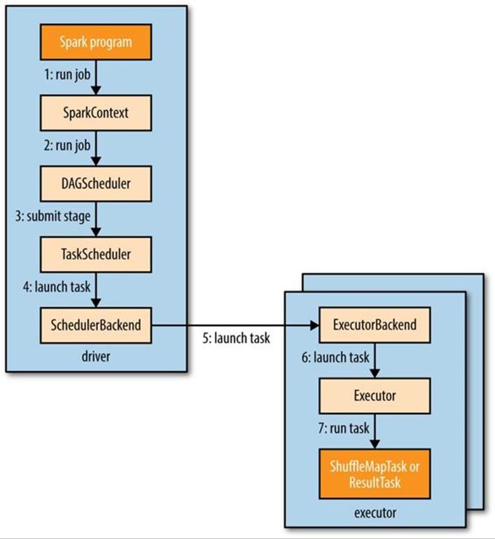
Figure 19-1. How Spark runs a job
Next, let’s take a look at how the DAG scheduler constructs a DAG.
DAG Construction
To understand how a job is broken up into stages, we need to look at the type of tasks that can run in a stage. There are two types: shuffle map tasks and result tasks. The name of the task type indicates what Spark does with the task’s output:
Shuffle map tasks
As the name suggests, shuffle map tasks are like the map-side part of the shuffle in MapReduce. Each shuffle map task runs a computation on one RDD partition and, based on a partitioning function, writes its output to a new set of partitions, which are then fetched in a later stage (which could be composed of either shuffle map tasks or result tasks). Shuffle map tasks run in all stages except the final stage.
Result tasks
Result tasks run in the final stage that returns the result to the user’s program (such as the result of a count()). Each result task runs a computation on its RDD partition, then sends the result back to the driver, and the driver assembles the results from each partition into a final result (which may be Unit, in the case of actions like saveAsTextFile()).
The simplest Spark job is one that does not need a shuffle and therefore has just a single stage composed of result tasks. This is like a map-only job in MapReduce.
More complex jobs involve grouping operations and require one or more shuffle stages. For example, consider the following job for calculating a histogram of word counts for text files stored in inputPath (one word per line):
val hist: Map[Int, Long] = sc.textFile(inputPath)
.map(word => (word.toLowerCase(), 1))
.reduceByKey((a, b) => a + b)
.map(_.swap)
.countByKey()
The first two transformations, map() and reduceByKey(), perform a word count. The third transformation is a map() that swaps the key and value in each pair, to give (count, word) pairs, and the final operation is the countByKey() action, which returns the number of words with each count (i.e., a frequency distribution of word counts).
Spark’s DAG scheduler turns this job into two stages since the reduceByKey() operation forces a shuffle stage.[131] The resulting DAG is illustrated in Figure 19-2.
The RDDs within each stage are also, in general, arranged in a DAG. The diagram shows the type of the RDD and the operation that created it. RDD[String] was created by textFile(), for instance. To simplify the diagram, some intermediate RDDs generated internally by Spark have been omitted. For example, the RDD returned by textFile() is actually a MappedRDD[String] whose parent is a HadoopRDD[LongWritable, Text].
Notice that the reduceByKey() transformation spans two stages; this is because it is implemented using a shuffle, and the reduce function runs as a combiner on the map side (stage 1) and as a reducer on the reduce side (stage 2) — just like in MapReduce. Also like MapReduce, Spark’s shuffle implementation writes its output to partitioned files on local disk (even for in-memory RDDs), and the files are fetched by the RDD in the next stage.[132]
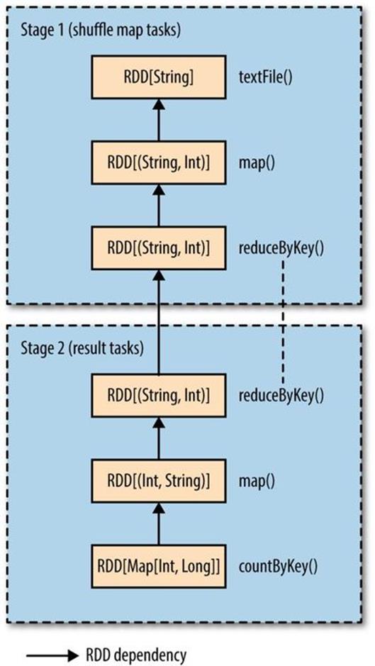
Figure 19-2. The stages and RDDs in a Spark job for calculating a histogram of word counts
If an RDD has been persisted from a previous job in the same application (SparkContext), then the DAG scheduler will save work and not create stages for recomputing it (or the RDDs it was derived from).
The DAG scheduler is responsible for splitting a stage into tasks for submission to the task scheduler. In this example, in the first stage one shuffle map task is run for each partition of the input file. The level of parallelism for a reduceByKey() operation can be set explicitly by passing it as the second parameter. If not set, it will be determined from the parent RDD, which in this case is the number of partitions in the input data.
Each task is given a placement preference by the DAG scheduler to allow the task scheduler to take advantage of data locality. A task that processes a partition of an input RDD stored on HDFS, for example, will have a placement preference for the datanode hosting the partition’s block (known as node local), while a task that processes a partition of an RDD that is cached in memory will prefer the executor storing the RDD partition (process local).
Going back to Figure 19-1, once the DAG scheduler has constructed the complete DAG of stages, it submits each stage’s set of tasks to the task scheduler (step 3). Child stages are only submitted once their parents have completed successfully.
Task Scheduling
When the task scheduler is sent a set of tasks, it uses its list of executors that are running for the application and constructs a mapping of tasks to executors that takes placement preferences into account. Next, the task scheduler assigns tasks to executors that have free cores (this may not be the complete set if another job in the same application is running), and it continues to assign more tasks as executors finish running tasks, until the task set is complete. Each task is allocated one core by default, although this can be changed by setting spark.task.cpus.
Note that for a given executor the scheduler will first assign process-local tasks, then node-local tasks, then rack-local tasks, before assigning an arbitrary (nonlocal) task, or a speculative task if there are no other candidates.[133]
Assigned tasks are launched through a scheduler backend (step 4 in Figure 19-1), which sends a remote launch task message (step 5) to the executor backend to tell the executor to run the task (step 6).
NOTE
Rather than using Hadoop RPC for remote calls, Spark uses Akka, an actor-based platform for building highly scalable, event-driven distributed applications.
Executors also send status update messages to the driver when a task has finished or if a task fails. In the latter case, the task scheduler will resubmit the task on another executor. It will also launch speculative tasks for tasks that are running slowly, if this is enabled (it is not by default).
Task Execution
An executor runs a task as follows (step 7). First, it makes sure that the JAR and file dependencies for the task are up to date. The executor keeps a local cache of all the dependencies that previous tasks have used, so that it only downloads them when they have changed. Second, it deserializes the task code (which includes the user’s functions) from the serialized bytes that were sent as a part of the launch task message. Third, the task code is executed. Note that tasks are run in the same JVM as the executor, so there is no process overhead for task launch.[134]
Tasks can return a result to the driver. The result is serialized and sent to the executor backend, and then back to the driver as a status update message. A shuffle map task returns information that allows the next stage to retrieve the output partitions, while a result task returns the value of the result for the partition it ran on, which the driver assembles into a final result to return to the user’s program.
Executors and Cluster Managers
We have seen how Spark relies on executors to run the tasks that make up a Spark job, but we glossed over how the executors actually get started. Managing the lifecycle of executors is the responsibility of the cluster manager, and Spark provides a variety of cluster managers with different characteristics:
Local
In local mode there is a single executor running in the same JVM as the driver. This mode is useful for testing or running small jobs. The master URL for this mode is local (use one thread), local[n] (n threads), or local(*) (one thread per core on the machine).
Standalone
The standalone cluster manager is a simple distributed implementation that runs a single Spark master and one or more workers. When a Spark application starts, the master will ask the workers to spawn executor processes on behalf of the application. The master URL isspark://host:port.
Mesos
Apache Mesos is a general-purpose cluster resource manager that allows fine-grained sharing of resources across different applications according to an organizational policy. By default (fine-grained mode), each Spark task is run as a Mesos task. This uses the cluster resources more efficiently, but at the cost of additional process launch overhead. In coarse-grained mode, executors run their tasks in-process, so the cluster resources are held by the executor processes for the duration of the Spark application. The master URL is mesos://host:port.
YARN
YARN is the resource manager used in Hadoop (see Chapter 4). Each running Spark application corresponds to an instance of a YARN application, and each executor runs in its own YARN container. The master URL is yarn-client or yarn-cluster.
The Mesos and YARN cluster managers are superior to the standalone manager since they take into account the resource needs of other applications running on the cluster (MapReduce jobs, for example) and enforce a scheduling policy across all of them. The standalone cluster manager uses a static allocation of resources from the cluster, and therefore is not able to adapt to the varying needs of other applications over time. Also, YARN is the only cluster manager that is integrated with Hadoop’s Kerberos security mechanisms (see Security).
Spark on YARN
Running Spark on YARN provides the tightest integration with other Hadoop components and is the most convenient way to use Spark when you have an existing Hadoop cluster. Spark offers two deploy modes for running on YARN: YARN client mode, where the driver runs in the client, and YARN cluster mode, where the driver runs on the cluster in the YARN application master.
YARN client mode is required for programs that have any interactive component, such as spark-shell or pyspark. Client mode is also useful when building Spark programs, since any debugging output is immediately visible.
YARN cluster mode, on the other hand, is appropriate for production jobs, since the entire application runs on the cluster, which makes it much easier to retain logfiles (including those from the driver program) for later inspection. YARN will also retry the application if the application master fails (see Application Master Failure).
YARN client mode
In YARN client mode, the interaction with YARN starts when a new SparkContext instance is constructed by the driver program (step 1 in Figure 19-3). The context submits a YARN application to the YARN resource manager (step 2), which starts a YARN container on a node manager in the cluster and runs a Spark ExecutorLauncher application master in it (step 3). The job of the ExecutorLauncher is to start executors in YARN containers, which it does by requesting resources from the resource manager (step 4), then launching ExecutorBackend processes as the containers are allocated to it (step 5).
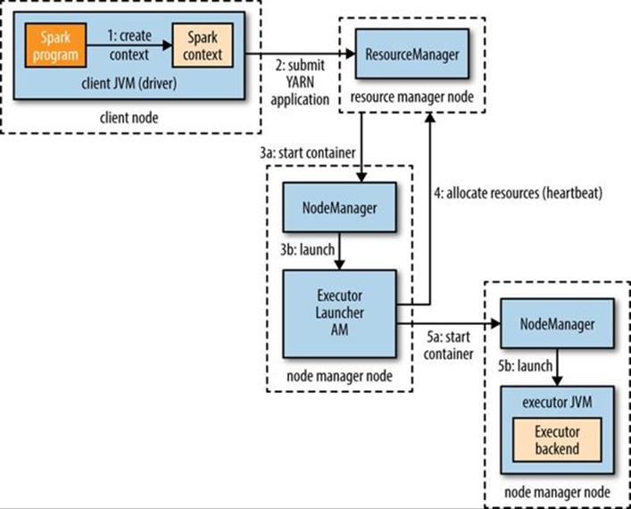
Figure 19-3. How Spark executors are started in YARN client mode
As each executor starts, it connects back to the SparkContext and registers itself. This gives the SparkContext information about the number of executors available for running tasks and their locations, which is used for making task placement decisions (described in Task Scheduling).
The number of executors that are launched is set in spark-shell, spark-submit, or pyspark (if not set, it defaults to two), along with the number of cores that each executor uses (the default is one) and the amount of memory (the default is 1,024 MB). Here’s an example showing how to run spark-shell on YARN with four executors, each using one core and 2 GB of memory:
% spark-shell --master yarn-client \
--num-executors 4 \
--executor-cores 1 \
--executor-memory 2g
The YARN resource manager address is not specified in the master URL (unlike when using the standalone or Mesos cluster managers), but is picked up from Hadoop configuration in the directory specified by the HADOOP_CONF_DIR environment variable.
YARN cluster mode
In YARN cluster mode, the user’s driver program runs in a YARN application master process. The spark-submit command is used with a master URL of yarn-cluster:
% spark-submit --master yarn-cluster ...
All other parameters, like --num-executors and the application JAR (or Python file), are the same as for YARN client mode (use spark-submit --help for usage).
The spark-submit client will launch the YARN application (step 1 in Figure 19-4), but it doesn’t run any user code. The rest of the process is the same as client mode, except the application master starts the driver program (step 3b) before allocating resources for executors (step 4).
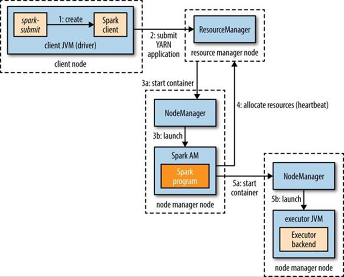
Figure 19-4. How Spark executors are started in YARN cluster mode
In both YARN modes, the executors are launched before there is any data locality information available, so it could be that they end up not being co-located on the datanodes hosting the files that the jobs access. For interactive sessions, this may be acceptable, particularly as it may not be known which datasets are going to be accessed before the session starts. This is less true of production jobs, however, so Spark provides a way to give placement hints to improve data locality when running in YARN cluster mode.
The SparkContext constructor can take a second argument of preferred locations, computed from the input format and path using the InputFormatInfo helper class. For example, for text files, we use TextInputFormat:
val preferredLocations = InputFormatInfo.computePreferredLocations(
Seq(new InputFormatInfo(new Configuration(), classOf[TextInputFormat],
inputPath)))
val sc = new SparkContext(conf, preferredLocations)
The preferred locations are used by the application master when making allocation requests to the resource manager (step 4).[135]
Further Reading
This chapter only covered the basics of Spark. For more detail, see Learning Spark by Holden Karau, Andy Konwinski, Patrick Wendell, and Matei Zaharia (O’Reilly, 2014). The Apache Spark website also has up-to-date documentation about the latest Spark release.
[128] See Matei Zaharia et al., “Resilient Distributed Datasets: A Fault-Tolerant Abstraction for In-Memory Cluster Computing,” NSDI ’12 Proceedings of the 9th USENIX Conference on Networked Systems Design and Implementation, 2012.
[129] The Java version is much more compact when written using Java 8 lambda expressions.
[130] This is like performing a parameter sweep using NLineInputFormat in MapReduce, as described in NLineInputFormat.
[131] Note that countByKey() performs its final aggregation locally on the driver rather than using a second shuffle step. This is unlike the equivalent Crunch program in Example 18-3, which uses a second MapReduce job for the count.
[132] There is scope for tuning the performance of the shuffle through configuration. Note also that Spark uses its own custom implementation for the shuffle, and does not share any code with the MapReduce shuffle implementation.
[133] Speculative tasks are duplicates of existing tasks, which the scheduler may run as a backup if a task is running more slowly than expected. See Speculative Execution.
[134] This is not true for Mesos fine-grained mode, where each task runs as a separate process. See the following section for details.
[135] The preferred locations API is not stable (in Spark 1.2.0, the latest release as of this writing) and may change in a later release.
All materials on the site are licensed Creative Commons Attribution-Sharealike 3.0 Unported CC BY-SA 3.0 & GNU Free Documentation License (GFDL)
If you are the copyright holder of any material contained on our site and intend to remove it, please contact our site administrator for approval.
© 2016-2026 All site design rights belong to S.Y.A.