Foundations of Algorithms (2015)

Chapter 10 Genetic Algorithms and Genetic Programming

Evolution is the process of change in the genetic makeup of populations. Natural selection is the process by which organisms possessing traits that better enable them to adapt to environmental pressures survive and reproduce in greater numbers than other similar organisms, thereby increasing the existence of those favorable traits in future generations.

Evolutionary computation endeavors to obtain approximate solutions to problems such as optimization problems using the evolutionary mechanisms involved in natural selection as its paradigm. The four areas of evolutionary computation are genetic algorithms, genetic programming, evolutionary programming, and evolutionary strategies. The first two areas are discussed in detail in the chapter. First, we briefly review genetics to provide a proper context for these algorithms.

10.1 Genetics Review

This brief review assumes that you have seen this material before. For an introduction to genetics, see An Introduction to Genetic Analysis (Griffiths et al., 2007) or Essential Genetics (Hartl and Jones, 2006).

An organism is an individual form of life such as a plant or animal. A cell is the basic structural and functional unit of an organism. Chromosomes are the carriers of biologically expressed hereditary characteristics. A genome is a complete set of chromosomes in an organism. The human genome contains 23 chromosomes. A haploid cell contains one genome; that is, it contains one set of chromosomes. So a human haploid cell contains 23 chromosomes. A diploid cell contains two genomes; that is, it contains two sets of chromosomes. Each chromosome in one set is matched with a chromosome in the other set. This pair of chromosomes is called a homologous pair. Each chromosome in the pair is called a homolog. So a human diploid cell contains 2 × 23 = 46 chromosomes. One homolog comes from each parent.

A somatic cell is one of the cells in the body of the organism. A haploid organism is an organism with somatic cells that are haploid. A diploid organism is an organism with somatic cells that are diploid. Humans are diploid organisms.

A gamete is a mature sexual reproductive cell that unites with another gamete to become a zygote, which eventually grows into a new organism. A gamete is always haploid. The gamete produced by a male is called a sperm, whereas the gamete that is produced by the female is called an egg.Germ cells are precursors of gametes. They are diploid.

In diploid organisms, each adult produces a gamete, the two gametes combine to form a zygote, and the zygote grows to become a new adult. This process is called sexual reproduction. Unicellular haploid organisms commonly reproduce asexually by a process called binary fission. The organism simply splits into two new organisms. So, each new organism has the exact same genetic content as the original organism. Some unicellular haploid organisms reproduce sexually by a process called fusion. Two adult cells first combine to form what is called a transient diploid meiocyte. The transient diploid meiocyte contains a homologous pair of chromosomes, one from each parent. A child can obtain a given homolog from each parent, so the children are not genetic copies of the parents. For example, if the genome size is 3, there are 2³ = 8 different chromosome combinations that a child could have.

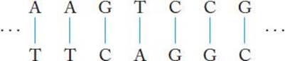
Chromosomes consist of the compound deoxyribonucleic acid (DNA). DNA is composed of four basic molecules called nucleotides. Each nucleotide contains a pentose sugar (deoxyribose), a phosphate group, and a purine or pyrimidine base. The purines, adenine (A) and guanine (G), are similar in structure, as are the pyrimidines, cytosine (C) and thymine (T). DNA is a macromolecule composed of two complementary strands, each of which consists of a sequence of nucleotides. The strands are joined together by hydrogen bonds between pairs of nucleotides. Adenine always pairs with thymine, and guanine always pairs with cytosine. Each such pair is called a canonical base pair (bp), and A, G, C, and T are called bases.

A section of DNA is depicted in Figure 10.1. You may recall from your biology course that the strands twist around each other to form a righthanded double helix. However, for our computational purposes, we need only consider them as character strings, as shown in Figure 10.1.

A gene is a section of a chromosome, often consisting of thousands of base pairs; the size of genes varies a great deal. Genes are responsible for both the structure and the processes of an organism. The genotype of an organism is its genetic makeup, while the phenotype of an organism is its appearance, which results from the interaction of the genotype and the environment.

Figure 10.1 A section of DNA.

An allele is any of several forms of a gene, usually arising through mutation. Alleles are responsible for hereditary variation.

Example 10.1

The bey2 gene on chromosome 15 is responsible for eye color in humans. There is one allele for blue eyes, which we call BLUE, and one for brown eyes, which we call BROWN. As is the case for all genes, an individual gets one allele from each parent. The BLUE allele is recessive. This means that if an individual receives one BLUE allele and one BROWN allele, that individual will have brown eyes. The only way the individual can have blue eyes is if the individual has two BLUE alleles. We also say that the brown allele is dominant.

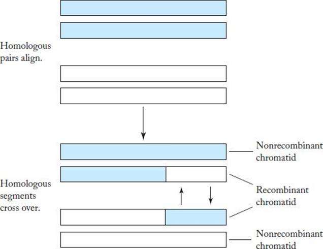
Because a human gamete has 23 chromosomes and each of these chromosomes can come from either genome, there are 2²³ = 8, 388, 608 different genetic combinations a parent can pass on to his or her offspring. Actually, there are many more than this. During meiosis (the cell division that produces gametes), each chromosome duplicates itself and aligns with its homolog. The duplicates are called chromatids. Often there is an exchange of corresponding segments of genetic material between the homologous chromatids facing each other. This exchange is called crossing-over and is illustrated in Figure 10.2.

Sometimes during cell division, errors occur in the DNA replication process. These errors are called mutations. Mutations can occur in either somatic cells or germ cells. It is believed that mutations in germ cells are the source of all variation in evolution. On the other hand, mutations in a somatic cell can affect an organism (e.g., cause cancer) but have no effect on its offspring.

In a substitution mutation, one nucleotide is simply replaced by another. An insertion mutation occurs when a section of DNA is added to a chromosome; a deletion mutation occurs when a section of DNA is removed from a chromosome.

Evolution is the process of change in the genetic makeup of populations. It is believed that the changes in genetic makeup are due to mutations. As noted earlier, natural selection is the process by which organisms possessing traits that better enable them to adapt to environmental pressures such as predators, changes in climate, or competition for food or mates will survive and reproduce in greater numbers than other similar organisms, thereby increasing the existence of those favorable traits in future generations. So, natural selection can result in an increase in the relative frequencies of alleles that impart these favorable traits to the individual. The process of the change in allele relative frequencies due to chance only is called genetic drift. There is some disagreement in the scientific community about whether natural selection or genetic drift is more responsible for evolutionary change (Li, 1997).

Figure 10.2 An illustration of crossing-over.

10.2 Genetic Algorithms

First, we describe the basic genetic algorithm; then, we provide two applications.

• 10.2.1 Algorithm

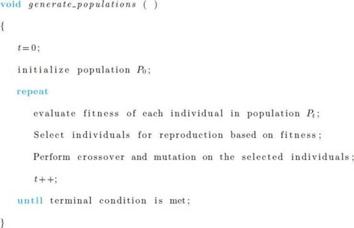
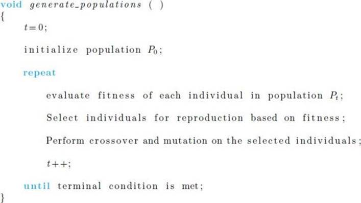
Genetic algorithms use fusion in haploid organisms as a model. Candidate solutions to a problem are represented by haploid individuals in a population. Each individual has one chromosome. The alphabet for the chromosome is not A, G, C, and T as in actual organisms, but rather consists of characters that represent solutions. In each generation, a certain number of fit individuals are allowed to reproduce. Individuals representing better solutions are more fit. The chromosomes from two fit individuals then line up and exchange genetic material (substrings of the problem solution) bycrossing-over. Furthermore, mutations may occur. This results in the next generation of individuals. The process is repeated until some terminal condition is met. The following is high-level pseudocode for a general genetic algorithm.

When selecting individuals based on fitness, we do not necessarily simply choose the most fit individuals. Rather, we may employ both exploitation and exploration. In general, when evaluating candidate regions of a search space to investigate, by exploitation we mean to exploit knowledge already obtained by concentrating on regions that look good; by exploration we mean looking for new regions without regard for how good they currently appear. In the case of choosing individuals, we could explore by choosing a random individual with probability and exploit by choosing a fit individual with probability 1 – .

• 10.2.2 Illustrative Example

Suppose our goal is to find the value of x that maximizes

where x is restricted to being an integer. Of course the sine function has its maximum value of 1 at π/2, which means x = 128 maximizes the function. Therefore, there is no practical reason to develop an algorithm to solve this problem. However, we do so to illustrate the various aspects of such algorithms. The following steps are used to develop the algorithm.

1. Choose an alphabet to represent solutions to the problem. Because candidate solutions are simply integers in the range 0 to 255, we can represent each individual (candidate solution) using 8 bits. For example, the integer 189 is represented as

2. Decide how many individuals make up a population. In general, there can be thousands of individuals. In this simple example, we will use 8 individuals.

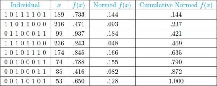
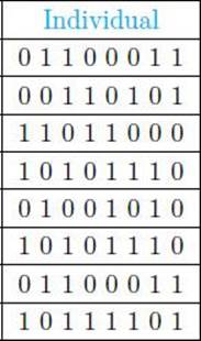
3. Decide how to initialize the population. Often this is done at random. We will generate 8 numbers at random from the range 0 to 255. Possible initial values appear in Table 10.1.

4. Decide how to evaluate fitness. Because our goal is to maximize f(x) = sin(xπ/256), the fitness of individual x is simply the value of this function.

5. Decide which individuals to select for reproduction. We will combine exploration with exploitation here. The fitnesses are normalized by dividing each fitness by the sum of all the fitnesses, which is 5.083, to yield normalized fitnesses. In this way, the normalized fitnesses add up to 1. These normalized fitnesses are then used to determine cumulative fitness values, which provide a wedge on a roulette wheel for each individual based on its fitness. This is shown in Table 10.1. For example, the second individual has a normalized fitness of .093 and that individual is assigned the wedge corresponding to the interval (.144, .237], which has width .093. We then generate a random number from the interval (0, 1]. That number will fall in the range assigned to precisely one individual, and this is the individual chosen. This process is performed 8 times.

• Table 10.1 Initial Population of Individuals and Their Fitnesses

Suppose the individuals chosen for reproduction are the ones that appear in Table 10.2. Note that an individual can appear more than once, and the likelihood of how often it appears depends on its fitness.

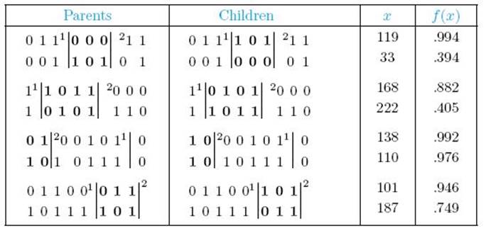
6. Determine how to perform crossovers and mutations. First, we randomly pair individuals, resulting in 4 pairs. For each pair, we randomly select two points along the individuals. Genetic material between the crossover points is exchanged. Table 10.3 shows possible results. Note that if the second point appears before the first point in the individual, crossover is performed by wrapping around. The third pair of individuals in Table 10.3 illustrates this case. Based on the values in Tables 10.1 and 10.3, the average fitness before crossover is .635, while that after crossover is .792. Furthermore, after crossover, two individuals have fitnesses above .99.

• Table 10.2 Individuals Chosen for Reproduction

• Table 10.3 Parents and Children Resulting from Crossover

Next, we determine how to perform mutations. For each bit in each individual, we decide at random whether to flip the bit (change 0 to 1 or 1 to 0). Mutation probabilities are commonly in the range .01 to .001.

7. Decide when to terminate. We can terminate when some maximum number of generations is attained, when some allotted amount of time has expired, when the fitness of the most fit individual reaches a certain level, or when one of these conditions is met. In this example, we can terminate when either 10,000 generations are produced or when the fitness exceeds .999.

Note that Steps 2, 3, 5, and 7 are generic in the sense that we can apply the strategies mentioned to most problems.

• 10.2.3 The Traveling Salesperson Problem

The Traveling Salesperson Problem (TSP) is a well-known NP-hard problem. NP-hard problems are a class of problems for which no one has ever developed a polynomial-time algorithm, but no one has ever shown that such an algorithm is not possible.

Suppose a salesperson is planning a sales trip to n cities. Each city is connected to some of the other cities by a road. To minimize travel time, we want to find a shortest route (called a tour) that starts at the salesperson’s home city, visits each of the cities once, and ends up at the home city. The problem of determining a shortest tour is the TSP. Note that the starting city is irrelevant to the shortest tour.

The TSP problem is represented by a weighted directed graph in which the vertices represent the cities and the weights on the edges represent road lengths. In general, the graph in an instance of the TSP need not be complete, meaning a graph in which there is an edge from every vertex to every other vertex. Furthermore, if the edges v_i → v_j and v_j → v_i are both in the graph, their weights need not be the same. In addition to application to transportation scheduling, the TSP has been applied to problems such as scheduling of a machine to drill holes in a circuit board and DNA sequencing.

Next, we show three genetic algorithms for the TSP.

Order Crossover

Order crossover is presented first. (Note: Only the steps that are different from those that appear Section 10.2.2 are shown).

1. Choose an alphabet to represent solutions to the problem. A straightforward representation of a solution to the TSP is to label the vertices 1 through n and list the vertices in the order visited. For example, if there are 9 vertices, [2 1 3 9 5 4 8 7 6] represents that we visit vertex v₁after v₂, v₃ afterv₂,…, and v₂ after v₆. Again, the starting vertex is irrelevant.

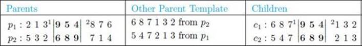
• Table 10.4 An Example of Order Crossover

4. The fitness is the length of the tour, where tours with shorter lengths are more fit.

6. Determine how to perform crossovers and mutations. As before, individuals are randomly paired and, for each pair, two points are randomly selected along the individuals. We call the segment between those points the pick. We must ensure the results of a crossover are legitimate tours, which means each city must be listed only once. Therefore, we cannot simply exchange picks. In order crossover, the pick in the child has the same value as the pick in the parent, whereas the nonpick area is filled in from values in the other parent, omitting values that are not already present, in the order in which those values appear in the other parent, starting from the other parent’s pick. These values are called its template. Table 10.4 illustrates this. Notice that child c₁ has value [9 5 4] for the pick, just as parent p₁. The pick for parent p₂ is [6 8 9]. The template from this parent is constructed by starting at site 6 and in sequence listing all cities that are not in [9 5 4]. This is done with wraparound. Thus, the template is [6 8 7 1 3 2]. These values are copied in order into the nonpick area of child c₂.
If the graph is not complete, we need to check whether the new child represents an actual tour, and if it does not, reject the crossover.
As far as mutations, we cannot just mutate a site by changing a given vertex to another vertex because a vertex would then appear twice. We can, however, mutate by interchanging two vertices or reversing the order of a subset of vertices. However, if the graph is not complete, we must make certain that the result represents an actual tour.

Nearest Neighbor Crossover

The Nearest Neighbor Algorithm (NNA) for the TSP is a greedy algorithm. The NNA starts with an arbitrary vertex to initiate a tour and then repeatedly adds the closest unvisited vertex to the partial tour until a tour is completed. The NNA assumes the graph is complete; otherwise it may not result in a tour. The algorithm follows.

Algorithm 10.1

Nearest Neighbor Algorithm (NNA) for the Traveling Salesperson Problem

Problem: Determine an optimal tour in a weighted, undirected graph. The weights are non-negative numbers.

Inputs: A weighted, undirected graph G, and n, the number of vertices in G.

Outputs: A variable tour containing an ordered list of the vertices in G.

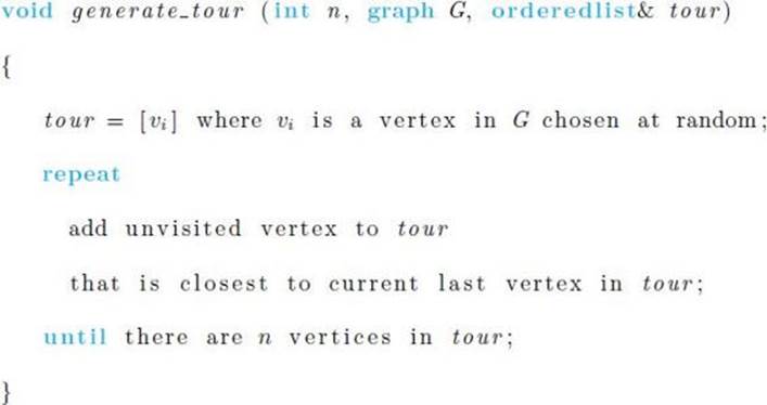
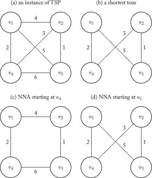
Figure 10.3(a) shows an instance of the TSP where the undirected edges represent that there is a directed edge with the given weight in both directions, Figure 10.3(b) shows the shortest tour, Figure 10.3(c) shows the tour obtained when we apply the NNA starting at v₄, and Figure 10.3(d) shows the tour obtained when we apply the NNA starting at v₁. Note that this latter tour is the optimal one.

Next, we present Nearest Neighbor Crossover (NNX), which was developed in 2010 by Süral et al. The steps shown are the ones used by those researchers when evaluating the algorithm.

1. Choose an alphabet to represent solutions to the problem. The representation is the same as that for order crossover, which appears at the beginning of Section 10.2.3.

2. Decide how many individuals make up a population. Population sizes of 50 and 100 were used.

3. One technique tried was to initialize the entire initial population at random. A second technique was to initialize half of the population at random and the other half using a hybrid technique involving NNX and the Greedy Edge Algorithm (discussed next).

4. Decide how to evaluate fitness. The fitness is the same as that for order crossover.

Figure 10.3 An instance of the TSP illustrating the NNA.

5. Decide which individuals to select for reproduction. The top 50% of individuals ordered according to fitness are allowed to reproduce. Four copies of each of these individuals are put in a pool. Then pairs of parents are randomly selected without replacement from the pool.

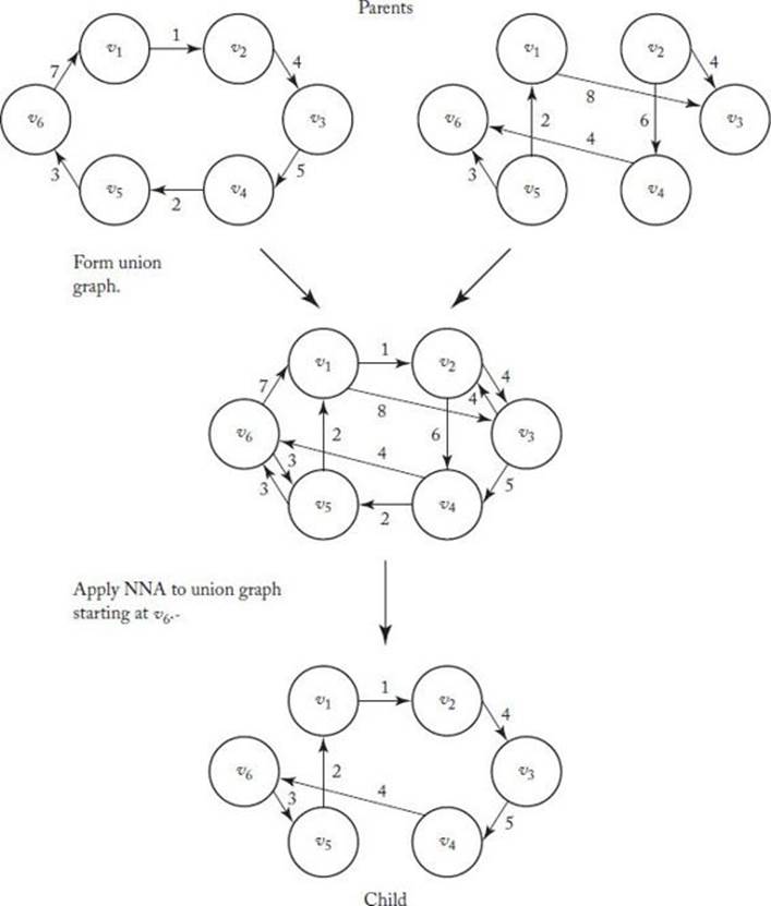
6. Determine how to perform crossovers and mutations. In NNX, two parents produce only one child. Therefore the process is not really crossover; nevertheless, we call it that. The parents first combine to form a union graph, which is a graph containing the edges in both parents. This process is illustrated in Figure 10.4. Then, NNA is applied to the union graph. This is also shown in Figure 10.4. In that figure, we applied NNA starting with vertex v₆, and we obtained a child that is more fit than either parent. Now we must also show that if we start at v₁, this does not happen. If we start at v₃, we reach a dead end at v₁and do not obtain a tour. If the chosen vertex does not result in a tour, we can try other vertices until one does. If no starting vertex results in a tour, we can make other edges in the complete graph eligible for our tour.
Note that because 4 copies of each parent are used and each pair of parents produces 1 offspring, the child generation is twice as large as the number of parents allowed to reproduce. However, because only half of the parents are allowed to do so, the size of the population stays the same in each generation.

Figure 10.4 The union graph is formed and then the NNA is applied to that graph starting a vertex v₆.

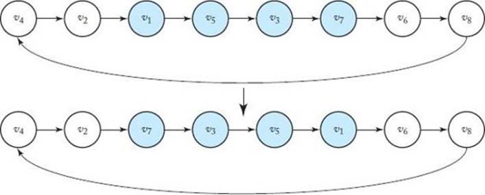
Mutations are performed as follows. Two vertices are selected at random, and the subpath connecting the two vertices is reversed. This is illustrated in Figure 10.5, where the vertices selected are v₁and v₇. There are two versions of mutation. In version M1, the mutation is applied only to the best offspring in each generation. In version M2, it is applied to all offspring.
As a variation, a stochastic version of NNX would choose the next edge incident to the current vertex probabilistically. The chance of being chosen would be inversely proportional to the length of the edge. It is possible to increase population diversity by doing this and thereby increase the portion of the search space investigated. However, Süral et al. (2010) found that this stochastic technique performed significantly worse than the deterministic version, and they did not include this in their final testing, which we discuss shortly.

Figure 10.5 A mutation in which the subpath connecting vertices v₁and v₇is reversed.

7. Decide when to terminate. The algorithm terminates when the average fitness in two successive generations is the same or when 500 generations are produced.

The NNA and NNX are very similar to Dikstra’s algorithm for the Shortest Paths Problem, and like that algorithm take θ(n²) time, where n is the number of vertices.

Greedy Edge Crossover

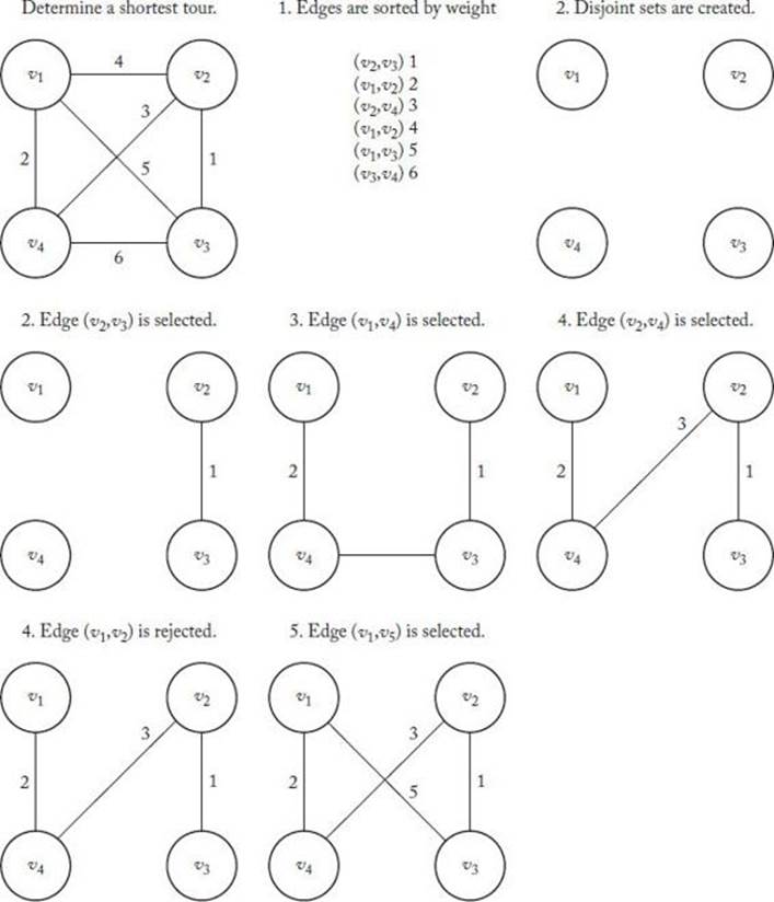
In the Greedy Edge Algorithm (GEA), we first sort the edges in nondecreasing sequence. We then greedily add edges to the tour, starting with the first edge, while making certain that no vertex has more than two edges touching it and that no cycle smaller than n is created. The GEA assumes the graph is complete; otherwise it may not result in a tour. The algorithm follows.

Algorithm 10.2

Greedy Edge Algorithm (GEA) for the Traveling Salesperson Problem

Problem: Determine an optimal tour in a weighted, undirected graph. The weights are non-negative numbers.

Inputs: A weighted, undirected graph G, and n, the number of vertices in G.

Outputs: A variable tour containing a set of edges in an optimal tour.

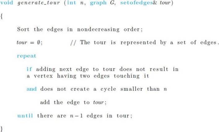
Figure 10.6 illustrates the GEA using the same instance as in Figure 10.3.

The Greedy Edge Crossover Algorithm (GEX) (also in Süral et al., 2010) has all the same steps as NNX except for the sixth step, which we show next.

6. Determine how to perform crossovers and mutations. As in NNX, in the GEX the parents first combine to form a union graph. Then the GEA is applied to the edges in this union graph. If this process does not result in a tour, the remaining edges in a tour are obtained by applying the GEA to the complete graph. This process, however, will result in little exploration and therefore high edge preservation and possible early convergence to a low-quality solution. To increase exploration, the first half of the new tour can be taken from the union graph and the second half from the complete graph. In initial investigations, this version performed much better than the one that took as many edges as possible from the union graph. This is the version that was used in the evaluation discussed next.

The NNA and NNX are very similar to Kruskal’s algorithm for the Minimum Spanning Tree Problem, and like that algorithm take θ(n²log n) and θ(m log m) time, where n is the number of vertices and m is the number of edges.

Figure 10.6 An instance of the TSP illustrating the Greedy Edge Algorithm.

Evaluation

As is the case for many heuristic algorithms, genetic algorithms do not have provably correct properties. Therefore, we evaluate them by investigating their performance on a number of instances of the problem. Süral et al. (2010) did this as follows for NNX and the GEX.

First, they obtained 10 instances of the TSP from the TSPLIB, which represent distances between real cities; the distances are symmetric (the same in both directions). The largest instance had n (the number of cities) = 226. They investigated versions of NNX and the GEX using no mutations,mutations M1 (discussed earlier), and mutations M2 (discussed earlier). Furthermore, they tried initialing the first population at random (R) and initializing using a hybrid technique (H) based on nearest neighbor and greedy edge heuristics. For each combination of mutation type and initialization type, they ran each of the algorithms 30 times on each of the 10 instances, making a total of 300 runs. The algorithm was coded in ANSIC and ran on a Pentium IV 1600 MHz machine with 256 MB RAM running RedHat Linux 8.0.

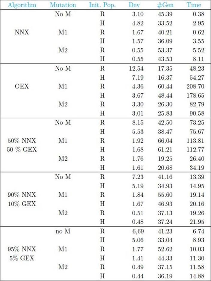
Table 10.5 shows the averages over all 300 runs. The headings in that table denote the following:

• Algorithm: The algorithm used.

• Mutation: The type of mutation used. “No M” denotes no mutations. • Init. Pop.: Whether the population was initialized at random (R) or using hybrid initialization (H).

• Dev: Percent deviation of the final best solution from the optimal solution.

• #Gen: Number of generations until convergence.

• Time: Time in seconds until convergence.

We see from Table 10.5 that NNX performed much better than the GEX, that mutation M2 performed the best of the mutations, and that hybrid initialization did not result in much better performance than random initialization. The researchers then investigated whether using NNX with various percentage usage of the GEX might improve performance. Table 10.5 also shows these results. When, for example, it says 50% NNX and 50% GEX, it means that 50% of the time the next population was generated using NNX and the other 50% of the time it was generated using the GEX. Slight improvement over pure NNX was observed in the case of mutation M2 for the higher percentages of NNX usage.

Based on these results, the researchers concluded that using mixtures of the two algorithms was not worth the increased computational time. Further experiments were performed using only NNX by itself.

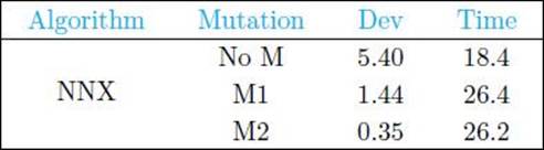
Using only NNX with random initialization but with a population size of 100, they obtained the results in Table 10.6. Note that for mutation M2, the average percent deviation is 0.35 and the average time is 26.2. Looking again at Table 10.5, we see that using this same combination with a population size of 50, the average percent deviation is 0.55 and the average time is 5.52. This increase in accuracy should be worth the increased time.

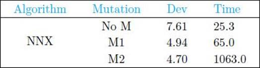
Next, the researchers investigated larger instances from the TSPLIB in which 318 ≤ n ≤ 1748. Having concluded that hybrid initialization is also not worth additional time, they ran NNX 10 times on each of these instances with random initialization and a population size of 100. Table 10.7shows the results. Curiously, on the large-problem instances, mutation M2 did not do much better than mutation M2 but required substantially more computation time. Looking again at Table 10.6, we see that in the case of small instances M2 performed much better than M1 with little increased computational cost.

• Table 10.5 Average Results Over 30 Runs on Each of 10 Small-Problem Instances Where Population Size Is 50

• Table 10.6 Average Results Over 30 Replications of 10 Small-Problem Instances Where Population Size Is 100 and the Initial Population Is Generated at Random

• Table 10.7 Average Results Over 10 Replications of 15 Large-Problem Instances Where Population Size Is 100 and Initial Population Is Generated at Random

• Table 10.8 A Comparison of NNX to Two Other Heurisic Algorithms for the TSP for 10 Problem Instances

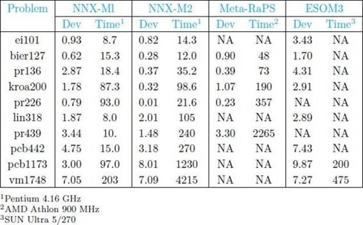
Simply testing a heuristic algorithm on a number of instances does not show if it as an advancement. We need to see how it fares relative to previously existing heuristic algorithms. Süral et al. (2010) compared NNX to the heuristic TSP algorithms Meta-RaPS (DePuy et al., 2005) and ESOM (Leung et al., 2004) using 10 benchmark TSP instances. Table 10.8 shows the results. Either NNX-M1 (mutation M1) or NNX-M2 (mutation M2) performed the best for every problem instance.

10.3 Genetic Programming

Whereas in genetic algorithms the “chromosome” or “individual” represents a solution to a problem, in genetic programing the individual represents a program that solves a problem. The fitness function for the individual in some way measures how well the program solves the problem. We start with an initial population of programs, allow the more fit programs to reproduce by crossover, perform mutations on the population of children, and then repeat this process until some terminal condition is met. The high-level algorithm for this procedure is exactly the same as the one for genetic algorithms. However, we show it next for completeness.

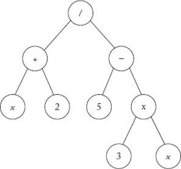
The individuals (programs) in a genetic program are represented by trees; in each node there is either a terminal symbol or a function symbol. If a node is a function symbol, its arguments are its children. As an example, suppose you have the following mathematical expression (program):

Its tree structure representation appears in Figure 10.7.

• 10.3.1 Illustrative Example

A simple way to illustrate genetic programming is to show an application that learns a function y = f(x) from pairs of points (x_i, y_i) known to satisfy the function. For example, suppose we have the pairs of points in Table 10.9.

Figure 10.7 A tree representing Equation 10.1.

These points were actually generated from the function

However, assume that we do not know this and are trying to discover the function. Steps for developing a genetic program for this discovery problem are as follows:

1. Decide on the terminal set T. Let the terminal set include the symbol x and the integers between −5 and 5.

2. Decide on the function set F. Let the function set be the symbols +, −, ×, and /. Note that we could include other functions such as sin, cos, etc. if desired.

3. Decide how many individuals make up a population. Our population size will be 600.

4. Decide how to initialize the population. Each initial individual is created by a process called growing the tree. First, a symbol is randomly generated from T ∪ F. If it is a terminal symbol, we stop and our tree consists of a single node containing this symbol. If it is a function symbol, we randomly generate children for the symbol. We continue down the tree, randomly generating symbols and stopping at terminal symbols. For example, the tree in Figure 10.7 would be obtained by the following random generation of symbols: First, the symbol / is generated, followed by the values of + and − for its children. The children generated for + are x and 2. We stop at each of these children. The children generated for − are 5 and ×. We stop at the 5, and finally generate the children 3 and x for the ×.

• Table 10.9 We Want to Learn a Function That Describes the Relationship between x and y Based on These 10 Points

5. Decide on a fitness function. The fitness function will be the square error. That is, the fitness of function f(x) is as follows:

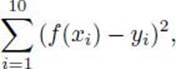
where each (x_i, y_i) is a point in Table 10.9. Functions with smaller errors are more fit.

6. Decide which individuals to select for reproduction. A 4-individual tournament selection process is used. In the tournament selection process, n individuals are randomly selected from the population. In this case, n = 4. We say that these n individuals enter a tournament in which the n/2 most fit of them win and the n/2 least fit lose. The n/2 winners are allowed to reproduce to produce n/2 children. These children replace the n/2 losers in the population for the next generation. In this case, the 2 winners reproduce twice to produce 2 children who replace the 2 losers.
A small tournament size results in low selection process, whereas a high tournament size results in high pressure.

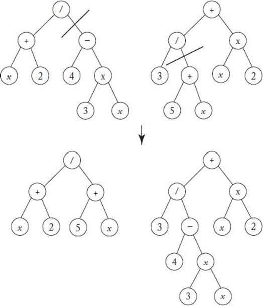
7. Decide how to perform crossovers and mutations. Crossover between two individuals will be performed by exchanging randomly selected subtrees. Such a crossover is illustrated in Figure 10.8. Mutations are performed by randomly selecting a node and replacing the subtree at that node by a growing a new subtree. Mutations are randomly performed on 5% of the offspring.

8. Decide when to terminate. Terminate when the square error of the most fit individual is 0 or when 100 generations have been produced.

Figure 10.8 Crossover by exchanging subtrees.

Banzhaf et al. (1998) applied the technique just presented to the data in Table 10.9. The following shows the most fit individual in the first 4 generations:

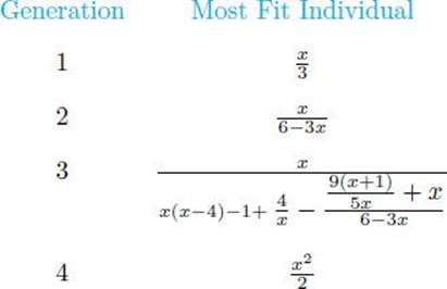
The most fit individual expanded to a very large tree by generation 3 but shrunk back down to the correct solution (the function generating the data) by generation 4.

• 10.3.2 Artificial Ant

Consider the problem of developing a robotic ant that navigates along a trail of food. Figure 10.9 shows such a trail, called the “Sante Fe trail.” Each black square represents one pellet of food; there are 89 such squares.

Figure 10.9 The Santa Fe trail. Each black square reprsents a pellet of food.

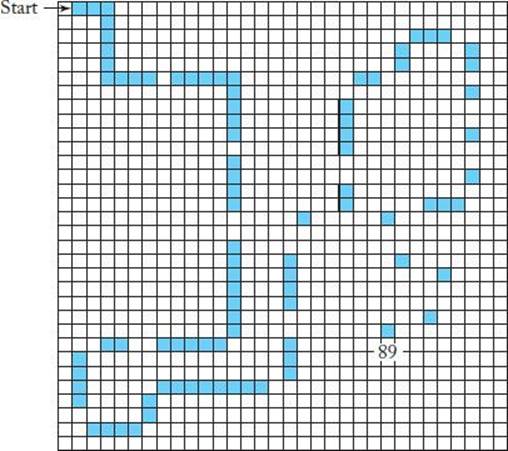
The ant starts at the square labeled “start” facing right, and its goal is to arrive at the square labeled “89” after visiting all 89 black squares (thereby eating all the food on the trail) in as few time steps as possible. Notice that there are a number of gaps along the trail. This problem in a example ofplanning problem.

The ant has one sensor as follows:

food_ahead: Has value True if there is food in the square the ant is facing; otherwise has value False.

There are three different actions the ant can execute in each time slot:

right: The ant turns right by 90^o(without moving).
left: The ant turns left by 90^o(without moving).
move: The ant moves forward into the square it is facing. If the square contains food, the ant eats the food, thereby eliminating the food from the square and erasing it from the trail.

Koza (1992) developed the following genetic programming algorithm for this problem.

1. Decide on the terminal set T. The terminal set contains the actions the ant can take. That is,

2. Decide on the function set F. The function set is as follows:
(a) if_food_ahead(instruction1, instruction2);
(b) do2(instruction1, instruction2);
(c) d03(instruction1, instruction2, instruction3);
The first function executes instruction1 if food ahead is true; otherwise it executes instruction2. The second function unconditionally executes instruction1 and instruction2. The third function unconditionally executes instruction1, instruction2, and instruction3. For example,

causes the ant to turn right and then move ahead.

3. Decide how many individuals make up a population. The population size is 500.

4. Decide how to initialize the population. Each initial individual is created by growing the tree (See Section 10.3.1).

5. Decide on a fitness function. It is assumed that each action (right, left, move) takes one time step, and each individual is allowed 400 time steps. Each individual starts in the upper left-hand square facing east. Fitness is defined as the number of food pellets consumed in the allotted time. The maximum fitness is 89.

6. Decide which individuals to select for reproduction.

7. Decide how to perform crossovers and mutations. Crossover between two individuals will be performed by exchanging randomly selected subtrees. Such a crossover is illustrated in Figure 10.8. Mutations are performed by randomly selecting a node and replacing the subtree at that node by growing a new subtree. Mutations are randomly performed on 5% of the offspring.

8. Decide when to terminate. Terminate when one individual has a fitness of 89 or some maximum amount of iterations is reached.

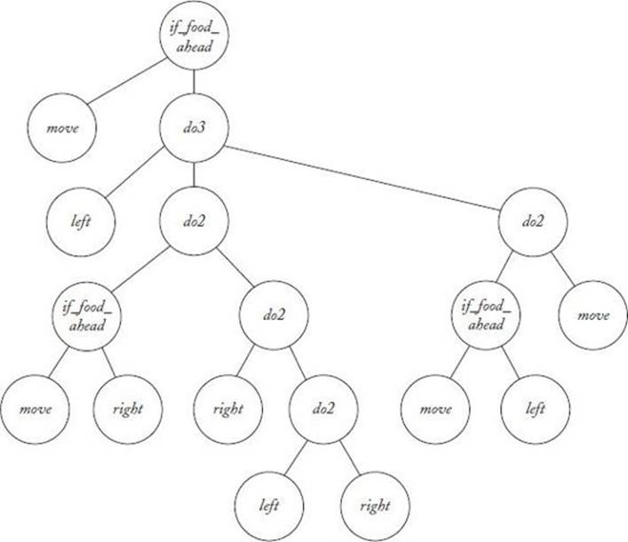
In each iteration, each individual in the population (program) is run repeatedly until 400 time steps are performed. The individual’s fitness is then evaluated. In one particular run, Koza (1992) obtained an individual with a fitness equal to 89 in the 22nd generation. That individual appears inFigure 10.10. The average fitness of individuals in generation 0 was 3.5, while the most fit individual in generation 0 had a fitness of 32.

• 10.3.3 Application to Financial Trading

An important decision facing everyone who invests in the stock and other financial markets is whether to buy, sell, or hold on a given day. There have been many efforts to develop automated systems that make this decision for us. Farnsworth et al. (2004) developed such a system using genetic programming. Their system makes an investment decision based on values of market indicators on a given day. We discuss that system next.

Figure 10.10 The individual in generation 22 with a fitness equal to 89.

Developing the Trading System

First, we show the eight steps used to create the system.

1. Decide on the terminal set T. The terminal symbols are the market indicators. The researchers tried and tested various indicators before deciding on the ones to include in the final system. We only present the final ones. They are as follows:

(a) The S&P 500 is a market index based on 500 leading companies in leading industries of the U.S. economy. For a given day, the indicator based on the S&P 500 is as follows:

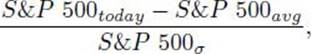
where S&P 500_todayis the value of the S&P500 on the current day, S&P 500_avgis the average value over the past 200 days, and S&P 500_σ is the standard deviation over the past 200 days.
We denote this indicator simply as SP 500.

(b) The k-day Exponential Moving Average (EMA) for a security is a weighted average of the security over the past k days.
The Moving Average Convergence/Divergence (MACD) of a security x is as follows:

The MACD is considered a momentum indicator. When it is positive, traders say upside momentum is increasing; when it is negative, they say downside momentum is increasing.
A second indicator used in this system is MACD(S&P 500), which we denote simply as MACD.

(c) The indicator MACD9 is the 9-day EMA of the MACD of the S&P 500.

(d) Let Diff be the difference of the number of advancing and declining securities. That McClennan Oscillator (MCCL) is as follows:

Traders consider the market overbought when MCCL > 100 and oversold when MCCL < −100.
We denote this indicator simply as MCCL

(e) The indicators SP 500lag, MACDlag, MACD9lag, and MCCLlag are the values of those indicators on the previous day.

(f) Other terminal symbols include real constants in the interval [−1, 1]. All indicator values were normalized to the interval [−1, 1].

2. Decide on the function set F. Function symbols include +, − and ×, and the following control structures:

(a) if x > 0 then y else z. This structure is represented in the tree with the symbol IF having the children x, y, and z.

(b) if x > w then y else z. This structure is represented in the tree with the symbol IFGT having the children x, w, y, and z.

3. Decide how many individuals make up a population. Various population sizes were tried. Sizes smaller than 500 were ineffectual, whereas ones around 2500 had good results.

4. Decide how to initialize the population. Each initial individual was created by growing the tree as discussed in Section 10.3.1. The maximum number of levels allowed was 4 and the maximum number of total nodes allowed was 24. This restriction was also enforced in future populations. The purpose of these limitations was to avoid overfitting, which occurs when the tree matches the training data very closely but has limited predictive value for unseen data.

5. Decide on a fitness function. Data was obtained on the S&P closing prices from April 4, 1983 to June 18, 2004. A given tree analyzes the first 4750 days of this data. The tree starts with $1 on the first day. If the tree returns a value greater than 0 on a given day, a buy signal is generated; otherwise a sell signal is generated. All the current money is always invested or withdrawn when there is a buy or a sell. There are no partial investments. If the tree was in the market on the previous day and a buy signal is generated, no action is taken. Similarly, if the tree was out of the market on the previous day and a sell signal is generated, no action is taken. When the 4750 days of trading are complete, the initial dollar is subtracted so that the final value represents profit. To further avoid overfitting, a fitness penalty proportional to the total number of transactions was imposed.

6. Decide which individuals to select for reproduction. The population is sorted according to fitness. The bottom 25% are “killed off” and replaced by more fit individuals.

7. Decide how to perform crossovers and mutations. Crossover between two individuals is performed by exchanging randomly selected subtrees. Node mutations are done by randomly selecting a few nodes and randomly changing their values to nodes that take the same arguments. Mutations to function nodes change operations, and mutations to terminal nodes change indicator or constant values. Tree mutations are performed by randomly selecting a subtree and replacing it by a new random subtree.
The top 10% of the population are left unchanged; 50% are randomly selected for crossover with individuals from the top 10%; 20% are selected for node mutations; 10% are selected for tree mutations; and 10% are killed and randomly replaced.

8. Decide when to terminate. The maximum number of generations was in the 300–500 range.

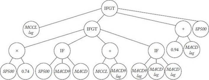
Figure 10.11 shows a tree that survived as the most fit tree in one particular run.

Figure 10.11 A tree that survived as most fit in one run and performed well in an evaluation.

Evaluation

Recall that data was obtained on the S&P closing prices from April 4, 1983 to June 18, 2004, and the first 4750 days of these data were used to determine the fitness and thereby learn a system. The remaining 500 days were used to evaluate a system by computing its fitness based on these data. The system represented by the tree in Figure 10.11 had an evaluation fitness of 0.397. The buy-and-hold strategy in investing is simply to buy a security and hold on to it. Based on the evaluation data, the buy-and-hold strategy only had a fitness of 0.1098.

10.4 Discussion and Further Reading

The remaining two areas of evolutionary computation are evolutionary programming and evolution strategies. Evolutionary programming is similar to genetic algorithms in that it uses a population of candidate solutions to evolve into an answer to a specific problem. Evolutionary programming differs in that its focus is on developing behavioral models of the observable systems interaction with the environment. Fogel (1994) presents this approach. Evolution strategies model problem solutions as species. Rechenberg (1994) says that the field of evolution strategies is based on the evolution of evolution. See Kennedy and Eberhart (2001) for a complete introduction to all four areas of evolutionary computation.

EXERCISES

Section 10.1

1. Describe the difference between sexual reproduction in diploid organisms, binary fission in haploid organisms, and fusion in haploid organisms.

2. Suppose a diploid organism has 10 chromosomes in one of its genomes.

(a) How many chromosomes are in each of its somatic cells?

(b) How many chromosomes are in each of its gametes?

3. Suppose two adult haploid organisms reproduce by fusion.

(a) How many children will be produced?

(b) Will the genetic content of the children all be the same?

4. Consider the eye color of a human being as determined by the bey2 gene. Recall that the allele for brown eyes is dominant. For each of the following parent allele combinations, determine the eye color of the individual.

Section 10.2

5. Consider Table 10.1. Suppose the fitnesses of the 8 individuals are .61, .23, .85, .11, .27, .36, .55, and .44. Compute the normed fitnesses and the cumulative normed fitnesses.

6. Suppose we perform basic crossover as illustrated in Table 10.3, the parents are 01101110 and 11010101, and the starting and ending points for crossover are 3 and 7. Show the two children produced.

7. Implement the genetic algorithm for finding the value of x that maximizes f(x) = sin(xπ/256), which is discussed in Section 10.2.2.

8. Consider the instance of the TSP in Figure 10.12. Assume the weights in both directions on an edge are the same. Find the shortest tour.

9. Suppose we perform order crossover, the parents are 3 5 2 1 4 6 8 7 9 and 5 3 2 6 9 1 8 7 4, and the starting and ending points for the pick are 4 and 7. Show the two children produced.

10. Consider the instance of the TSP in Figure 10.12. Apply the Nearest Neighbor Algorithm starting with each of the vertices. Do any of them yield the shortest tour?

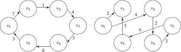
11. Form the union graph of the two tours shown in Figure 10.13, and apply the Nearest Neighborhood Algorithm to the resultant graph starting at vertex v₅.

12. Apply the Greedy Edge Algorithm to the instance of the TSP in Figure 10.12. Does it yield a shortest tour?

Figure 10.12 An instance of TSP.

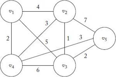
Figure 10.13 Two tours.

Section 10.3

13. Consider the two trees in Figure 10.8. Show the new trees that would be obtained if we exchanged the subtree starting with the “4” in the left tree with the subtree starting with the “+” in the right tree.

14. Consider the individual (program) in Figure 10.10. Show the moves produced by that program when negotiating the Santa Fe trail for the first 10 time steps.

15. Implement the genetic programming algorithm for the Santa Fe trail discussed in Section 10.3.2.