Foundations of Algorithms (2015)

Chapter 9 Computational Complexity and Intractability: An Introduction to the Theory of NP

Consider the following scenario based on a story in Garey and Johnson (1979). Suppose you work in industry, and your boss gives you the task of finding an efficient algorithm for some problem very important to the company. After laboring long hours on the problem for over a month, you make no headway at all toward an efficient algorithm. Giving up, you return to your boss and ashamedly announce that you simply can’t find an efficient algorithm. Your boss threatens to fire you and replace you with a smarter algorithm designer. You reply that perhaps it is not that you’re stupid, but rather that an efficient algorithm is not possible. Reluctantly, your boss gives you another month to prove that this is the case. After a second month of burning the midnight oil trying to prove this, you are unsuccessful. At this point you’ve failed to obtain an efficient algorithm and you’ve failed to prove that such an algorithm is not possible. You are on the verge of being fired, when you recall that some of the greatest computer scientists have worked on creating an efficient algorithm for the Traveling Salesperson problem, but nobody has ever developed one whose worst-case time complexity is better than exponential. Furthermore, no one has ever proven that such an algorithm is not possible. You see one last glimmer of hope. If you could prove that an efficient algorithm for the company’s problem would automatically yield an efficient algorithm for the Traveling Salesperson problem, it would mean that your boss is asking you to accomplish something that has eluded some of the greatest computer scientists. You ask for a chance to prove this, and your boss reluctantly agrees. After only a week of effort, you do indeed prove that an efficient algorithm for the company’s problem would automatically yield an efficient algorithm for the Traveling Salesperson problem. Rather than being fired, you’re given a promotion because you have saved the company a lot of money. Your boss now realizes that it would not be prudent to continue to expend great effort looking for an exact algorithm for the company’s problem and that other avenues, such as looking for an approximate solution, should be explored.

What we have just described is exactly what computer scientists have successfully done for the last 25 years. We have shown that the Traveling Salesperson problem and thousands of other problems are equally hard in the sense that if we had an efficient algorithm for any one of them, we would have efficient algorithms for all of them. Such an algorithm has never been found, but it’s never been proven that one is not possible. These interesting problems are called NP-complete and are the focus of this chapter. A problem for which an efficient algorithm is not possible is said to be “intractable.” In Section 9.1 we explain more concretely what it means for a problem to be intractable. Section 9.2 shows that when we are concerned with determining whether or not a problem is intractable, we must be careful about what we call the input size in an algorithm. Section 9.3 discusses three general categories in which problems can be grouped as far as intractability is concerned. The culmination of this chapter, Section 9.4, discusses the theory of NP and NP-complete problems. Section 9.5 shows ways of handling NP-complete problems.

9.1 Intractability

The dictionary defines intractable as “difficult to treat or work.” This means that a problem in computer science is intractable if a computer has difficulty solving it. This definition is too vague to be of much use to us. To make the notion more concrete, we now introduce the concept of a “polynomial-time algorithm.”

Definition

A polynomial-time algorithm is one whose worst-case time complexity is bounded above by a polynomial function of its input size. That is, if n is the input size, there exists a polynomial p (n) such that

Example 9.1

Algorithms with the following worst-case time complexities are all polynomial-time.

Algorithms with the following worst-case time complexities are not polynomial-time.

Notice that n lg n is not a polynomial in n. However, because

it is bounded by a polynomial in n, which means that an algorithm with this time complexity satisfies the criterion to be called a polynomial-time algorithm.

In computer science, a problem is called intractable if it is impossible to solve it with a polynomial-time algorithm. We stress that intractability is a property of a problem; it is not a property of any one algorithm for that problem. For a problem to be intractable, there must be no polynomial-time algorithm that solves it. Obtaining a nonpolynomial-time algorithm for a problem does not make it intractable. For example, the brute-force algorithm for the Chained Matrix Multiplication problem (see Section 3.4) is nonpolynomial-time. So is the divide-and-conquer algorithm that uses the recursive property established in Section 3.4. However, the dynamic programming algorithm (Algorithm 3.6) developed in that section is Θ (n³)_. The problem is not intractable, because we can solve it in polynomial-time using Algorithm 3.5.

In Chapter 1 we saw that polynomial-time algorithms are usually much better than algorithms that are not polynomial-time. Looking again at Table 1.4, we see that if it takes 1 nanosecond to process the basic instructions, an algorithm with a time complexity of n³ will process an instance of size 100 in 1 millisecond, whereas an algorithm with a time complexity of 2ⁿ will take billions of years.

We can create extreme examples in which a nonpolynomial-time algorithm is better than a polynomial-time algorithm for practical input sizes. For example, if n = 1, 000, 000,

Furthermore, many algorithms whose worst-case time complexities are not polynomials have efficient running times for many actual instances. This is the case for many backtracking and branch-and-bound algorithms. Therefore, our definition of intractable is only a good indication of real intractability. In any particular case, a problem for which we have found a polynomial-time algorithm could possibly be more difficult to handle, as far as practical input sizes are concerned, than one for which we cannot find such an algorithm.

There are three general categories of problems as far as intractability is concerned:

1. Problems for which polynomial-time algorithms have been found

2. Problems that have been proven to be intractable

3. Problems that have not been proven to be intractable, but for which polynomial-time algorithms have never been found

It is a surprising phenomenon that most problems in computer science seem to fall into either the first or third category.

When we are determining whether an algorithm is polynomial-time, it is necessary to be careful about what we call the input size. Therefore, before proceeding, let’s discuss the input size further. (See Section 1.3 for our initial discussion of the input size.)

9.2 Input Size Revisited

So far it has usually sufficed to call n the input size in our algorithms because n has been a reasonable measure of the amount of data in the input. For example, in the case of sorting algorithms, n, the number of keys to be sorted, is a good measure of the amount of data in the input. So we called nthe input size. However, we must not inadvertently call n the input size in an algorithm. Consider the following algorithm, which determines whether a positive integer n is prime.

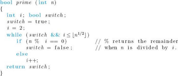
The number of passes through the while loop in this prime-checking algorithm is clearly in Θ(n^½). However, is it a polynomial-time algorithm? The parameter n is the input to the algorithm; it is not the size of the input. That is, each value of n constitutes an instance of the problem. This is unlike a sorting algorithm, for example, in which n is the number of keys and the instance is the n keys. If the value of n is the input and not the size of the input in function prime, what is the size of the input? We return to this question after we define input size more concretely than we did in Section 1.3.

Definition

For a given algorithm, the input size is defined as the number of characters it takes to write the input.

This definition is not different from that given in Section 1.3. It is only more specific about how we measure the size of the input. To count the characters it takes to write the input, we need to know how the input is encoded. Suppose that we encode it in binary, which is used inside computers. Then the characters used for the encoding are binary digits (bits), and the number of characters it takes to encode a positive integer x is lg x + 1. For example, 31 = 11111₂ and lg 31 + 1 = 5. We simply say that it takes about lg x bits to encode a positive integer x in binary. Suppose that we use binary encoding and we wish to determine the input size for an algorithm that sorts n positive integers. The integers to be sorted are the inputs to the algorithm. Therefore, the input size is the count of the number of bits it takes to encode them. If the largest integer is L, and we encode each integer in the number of bits needed to encode the largest, then it takes about lg L bits to encode each of them. The input size for the n integers is therefore about n lg L. Suppose that instead we choose to encode the integers in base 10. Then the characters used for the encoding are decimal digits, it takes about log L characters to encode the largest, and the input size for the n integers is about n log L. Because

an algorithm is polynomial-time in terms of one of these input sizes if and only if it is polynomial-time in terms of the other.

If we restrict ourselves to “reasonable” encoding schemes, then the particular encoding scheme used does not affect the determination of whether an algorithm is polynomial-time. There does not seem to be a satisfactory formal definition of “reasonable.” However, for most algorithms we usually agree on what is reasonable. For example, for any algorithm in this text, any base other than 1 could be used to encode an integer without affecting whether or not the algorithm is polynomial-time. We would therefore consider any such encoding system to be reasonable. Encoding in base 1, which is called the unary form, would not be considered reasonable.

In the preceding chapters, we simply called n, the number of keys to be sorted, the input size in our sorting algorithms. Using n as the input size, we showed that the algorithms are polynomial-time. Do they remain polynomial-time when we are precise about the input size? Next we illustrate that they do. When we are being precise about input size, we also need to be more precise (than we were in Section 1.3.1) about the definition of worst-case time complexity. The precise definition follows.

Definition

For a given algorithm, W (s) is defined as the maximum number of steps done by the algorithm for an input size of s. W (s) is called the worst-case time complexity of the algorithm.

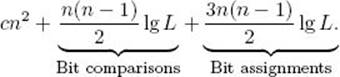
A step can be considered the equivalent of one machine comparison or assignment, or, to keep the analysis machine-independent, one bit comparison or assignment. This definition is not different from that given in Section 1.3. It is only more specific about the basic operation. That is, according to this definition, each step constitutes one execution of the basic operation. We used s instead of n for the input size because (1) the parameter n to our algorithms is not always a measure of the input size (e.g., in the prime-checking algorithm presented at the start of this section) and (2) when n is a measure of the input size, it is not ordinarily a precise measure of it. According to the definition just given, we must count all the steps done by the algorithm. Let’s illustrate how we can do this, while still avoiding the details of the implementation, by analyzing Algorithm 1.3 (Exchange Sort). For simplicity, assume that the keys are positive integers and that there are no other fields in the records. Look again at Algorithm 1.3. The number of steps done to increment loops and do branching is bounded by a constant c times n². If the integers are sufficiently large, they cannot be compared or assigned in one step by the computer. We saw a similar situation when we discussed large integer arithmetic in Section 2.6. Therefore, we should not consider one key comparison or assignment as one step. To keep our analysis machine-independent, we consider one step to be either one bit comparison or one bit assignment. Therefore, if L is the largest integer, it takes at most lg L steps to compare one integer or to assign one integer. When we analyzed Algorithm 1.3 in Sections 1.3 and 7.2, we saw that in the worst-case Exchange Sort does n (n − 1) 2 comparisons of keys and 3n (n − 1) /2 assignments to sort n positive integers. Therefore, the maximum number of steps done by Exchange Sort is no greater than

Let’s use s = n lg L as the input size. Then

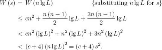
We have shown that Exchange Sort remains polynomial-time when we are precise about the input size. We can obtain similar results for all the algorithms, which we’ve shown to be polynomial-time using imprecise input sizes. Furthermore, we can show that the algorithms, which we’ve shown to be nonpolynomial-time (e.g., Algorithm 3.11), remain nonpolynomial-time when we are precise about the input size. We see that when n is a measure of the amount of data in the input, we obtain correct results concerning whether an algorithm is polynomial-time by simply using n as the input size. Therefore, when this is the case, we continue to use n as the input size.

We return now to the prime-checking algorithm. Because the input to the algorithm is the value of n, the input size is the number of characters it takes to encode n. Recall that if we are using base 10 encoding, it takes log n + 1 characters to encode n. For example, if the number is 340, it takes 3 decimal digits, not 340, to encode it. In general, if we are using base 10 encoding, and if we set

then s is approximately the size of the input. In the worst-case, there are n^1/2 − 1 passes through the loop in function prime. Because n = 10^s, the worst-case number of passes through the loop is about 10^s/2. Because the total number of steps is at least equal to the number of passes through the loop, the time complexity is nonpolynomial. If we use binary encoding, it takes about lg n characters to encode n. Therefore, if we use binary encoding,

is about equal to the input size, and the number of passes through the loop is about equal to 2^r/2. The time complexity is still nonpolynomial. The result remains unchanged as long as we use a “reasonable” encoding scheme. We mentioned previously that we would not consider unary encoding “reasonable.” If we used that encoding scheme, it would take n characters to encode the number n. For example, the number 7 would be encoded as 1111111. Using this encoding, the prime-checking algorithm has a polynomial time complexity. So we see that our results do change if we stray from a “reasonable” encoding system.

In algorithms such as the prime-checking algorithm, we call n a magnitude in the input. We’ve seen other algorithms whose time complexities are polynomials in terms of magnitude(s) but are not polynomials in terms of size. The time complexity of Algorithm 1.7 for computing the nth Fibonacci term is in Θ(n). Because n is a magnitude in the input and lg n measures the size of the input, the time complexity of Algorithm 1.7 is linear in terms of magnitudes but exponential in terms of size. The time complexity of Algorithm 3.2 for computing the binomial coefficient is in Θ(n²). Because n is a magnitude in the input and lg n measures the size of the input, the time complexity of Algorithm 3.2 is quadratic in terms of magnitudes but exponential in terms of size. The time complexity of the dynamic programming algorithm for the 0-1 Knapsack problem discussed in Section 4.5.4 is in Θ(nW). In this algorithm, n is a measure of size because it is the number of items in the input. However, W is a magnitude because it is the maximum capacity of the knapsack; lgW measures the size of W. This algorithm’s time complexity is polynomial in terms of magnitudes and size, but it is exponential in terms of size alone.

An algorithm whose worse-case time complexity is bounded above by a polynomial function of its size and magnitudes is called pseudopolynomialtime. Such an algorithm can often be quite useful because it is inefficient only when confronted with instances containing extremely large numbers. Such instances might not pertain to the application of interest. For example, in the 0-1 Knapsack problem, we might often be interested in cases where W is not extremely large.

9.3 The Three General Problem Categories

Next we discuss the three general categories in which problems can be grouped as far as intractability is concerned.

• 9.3.1 Problems for Which Polynomial-Time Algorithms Have Been Found

Any problem for which we have found a polynomial-time algorithm falls in this first category. We have found Θ(n lg n) algorithms for sorting, a Θ(lg n) algorithm for searching a sorted array, a Θ(n^2.38) algorithm for matrix multiplication, a Θ(n³) algorithm for chained matrix multiplication, and so on. Because n is a measure of the amounts of data in the inputs to these algorithms, they are all polynomial-time. The list goes on and on. There are algorithms that are not polynomial-time for many of these problems. We’ve already mentioned that this is the case for the Chained Matrix Multiplication algorithm. Other problems for which we have developed polynomial-time algorithms, but for which the obvious brute-force algorithms are nonpolynomial, include the Shortest Paths problem, the Optimal Binary Search Tree problem, and the Minimum Spanning Tree problem.

• 9.3.2 Problems That Have Been Proven to Be Intractable

There are two types of problems in this category. The first type are problems that require a nonpolynomial amount of output. Recall from Section 5.6 the problem of determining all Hamiltonian Circuits. If there was an edge from every vertex to every other vertex, there would be (n − 1)! such circuits. To solve the problem, an algorithm would have to output all of these circuits, which means that our request is not reasonable. We noted in Chapter 5 that we were stating the problems so as to ask for all solutions because we could then present less-cluttered algorithms, but that each algorithm could easily be modified to solve the problem that asks for only one solution. The Hamiltonian Circuits problem that asks for only one circuit clearly is not a problem of this type. Although it is important to recognize this type of intractability, problems such as these ordinarily pose no difficulty. It is usually straightforward to recognize that a nonpolynomial amount of output is being requested, and once we recognize this, we realize that we are simply asking for more information than we could possibly use. That is, the problem is not defined realistically.

The second type of intractability occurs when our requests are reasonable (that is, when we are not asking for a nonpolynomial amount of output) and we can prove that the problem cannot be solved in polynomial time. Oddly enough, we have found relatively few such problems. The first ones were undecidable problems. These problems are called “undecidable” because it can be proven that algorithms that solve them cannot exist. The most well-known of these is the Halting problem. In this problem we take as input any algorithm and any input to that algorithm, and decide whether or not the algorithm will halt when applied to that input. In 1936, Alan Turing showed that this problem is undecidable. In 1953, A. Grzegorczyk developed a decidable problem that is intractable. Similar results are discussed in Hartmanis and Stearns (1965). However, these problems were “artificially” constructed to have certain properties. In the early 1970s, some natural decidable decision problems were proven to be intractable. The output for a decision problem is a simple “yes” or “no” answer. Therefore, the amount of output requested is certainly reasonable. One of the most well-known of these problems is Presburger Arithmetic, which was proven intractable by Fischer and Rabin in 1974. This problem, along with the proof of intractability, can be found in Hopcroft and Ullman (1979).

All problems that to this date have been proven intractable have also been proven not to be in the set NP, which is discussed in Section 9.4. However, most problems that appear to be intractable are in the set NP. We discuss these problems next. As noted earlier, it is a somewhat surprising phenomenon that relatively few problems have been proven to be intractable, and it was not until the early 1970s that a natural decidable problem was proven intractable.

• 9.3.3 Problems That Have Not Been Proven to Be Intractable but for Which Polynomial-Time Algorithms Have Never Been Found

This category includes any problem for which a polynomial-time algorithm has never been found, but yet no one has ever proven that such an algorithm is not possible. As already discussed, there are many such problems. For example, if we state the problems so as to require one solution, the 0-1 Knapsack problem, the Traveling Salesperson problem, the Sum-of-Subsets problem, the m-Coloring problem for m ≥ 3, the Hamiltonian Circuits problem, and the problem of abductive inference in a Bayesian network all fall into this category. We have found branch-and-bound algorithms, backtracking algorithms, and other algorithms for these problems that are efficient for many large instances. That is, there is a polynomial in n that bounds the number of times the basic operation is done when the instances are taken from some restricted subset. However, no such polynomial exists for the set of all instances. To show this, we need only find some infinite sequence of instances for which no polynomial in n bounds the number of times the basic operation is done. Recall that we did this for the backtracking algorithms in Chapter 5.

There is a close and interesting relationship among many of the problems in this category. The development of this relationship is the purpose of the next section.

9.4 The Theory of NP

It is more convenient to develop the theory if we originally restrict ourselves to decision problems. Recall that the output of a decision problem is a simple “yes” or “no” answer. Yet when we introduced (in Chapters 3, 4, 5, and 6) some of the problems mentioned previously, we presented them as optimization problems, which means that the output is an optimal solution. Each optimization problem, however, has a corresponding decision problem, as the examples that follow illustrate.

Example 9.2

Traveling Salesperson Problem

Let a weighted, directed graph be given. Recall that a tour in such a graph is a path that starts at one vertex, ends at that vertex, and visits all the other vertices in the graph exactly once, and that the Traveling Salesperson Optimization problem is to determine a tour with minimal total weight on its edges.

The Traveling Salesperson Decision problem is to determine for a given positive number d whether there is a tour having total weight no greater than d. This problem has the same parameters as the Traveling Salesperson Optimization problem plus the additional parameter d.

Example 9.3

0-1 Knapsack Problem

Recall that the 0-1 Knapsack Optimization problem is to determine the maximum total profit of the items that can be placed in a knapsack given that each item has a weight and a profit, and that there is a maximum total weight W that can be carried in the sack.

The 0-1 Knapsack Decision problem is to determine, for a given profit P, whether it is possible to load the knapsack so as to keep the total weight no greater than W, while making the total profit at least equal to P. This problem has the same parameters as the 0-1 Knapsack Optimization problem plus the additional parameter P.

Example 9.4

Graph-Coloring Problem

The Graph-Coloring Optimization problem is to determine the minimum number of colors needed to color a graph so that no two adjacent vertices are colored the same color. That number is called the chromatic number of the graph.

The Graph-Coloring Decision problem is to determine, for an integer m, whether there is a coloring that uses at most m colors and that colors no two adjacent vertices the same color. This problem has the same parameters as the Graph-Coloring Optimization problem plus the additional parameter m.

Example 9.5

Clique Problem

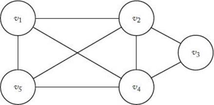
A clique in an undirected graph G = (V, E) is a subset W of V such that each vertex in W is adjacent to all the other vertices in W. For the graph in Figure 9.1, {v₂, v₃, v₄} is a clique, whereas {v₁, v₂, v₃} is not a clique because v₁ is not adjacent to v₃. A maximal clique is a clique of maximal size. The only maximal clique in the graph in Figure 9.1 is {v₁, v₂, v₄, v₅}.

The Clique Optimization problem is to determine the size of a maximal clique for a given graph.

The Clique Decision problem is to determine, for a positive integer k, whether there is a clique containing at least k vertices. This problem has the same parameters as the Clique Optimization problem plus the additional parameter k.

We have not found polynomial-time algorithms for either the decision problem or the optimization problem in any of these examples. However, if we could find a polynomial-time algorithm for the optimization problem in any one of them, we would also have a polynomial-time algorithm for the corresponding decision problem. This is so because a solution to an optimization problem produces a solution to the corresponding decision problem. For example, if we learned that the total weight of an optimal tour for a particular instance of the Traveling Salesperson Optimization problem was 120, the answer to the corresponding decision problem would be “yes” for

Figure 9.1 The maximal clique is {v₁, v₂, v₄, v₅}.

and “no” otherwise. Similarly, if we learned that the optimal profit for an instance of the 0-1 Knapsack Optimization problem was $230, the answer to the corresponding decision problem would be “yes” for

and “no” otherwise.

Because a polynomial-time algorithm for an optimization problem automatically produces a polynomial-time algorithm for the corresponding decision problem, we can initially develop our theory considering only decision problems. We do this next, after which we return to optimization problems. At that time, we will see that usually we can show that an optimization problem is even more closely related to its corresponding decision problem. That is, for many decision problems (including the problems in the previous examples), it’s been shown that a polynomial-time algorithm for the decision problem would yield a polynomial-time algorithm for the corresponding optimization problem.

• 9.4.1 The Sets P and NP

First we consider the set of decision problems that can be solved by polynomial-time algorithms. We have the following definition.

Definition

P is the set of all decision problems that can be solved by polynomial-time algorithms.

What problems are in P? All decision problems for which we have found polynomial-time algorithms are certainly in P. For example, the problem of determining whether a key is present in an array, the problem of determining whether a key is present in a sorted array, and the decision problems corresponding to the optimization problems in Chapters 3 and 4 for which we have found polynomial-time algorithms, are all in P. However, could some decision problem for which we have not found a polynomial-time algorithm also be in P? For example, could the Traveling Salesperson Decision problem be in P? Even though no one has ever created a polynomial-time algorithm that solves this problem, no one has ever proven that it cannot be solved with a polynomial-time algorithm. Therefore, it could possibly be in P. To know that a decision problem is not in P, we have toprove that it is not possible to develop a polynomial-time algorithm for it. This has not been done for the Traveling Salesperson Decision problem. These same considerations hold for the other decision problems in Examples 9.2 to 9.5.

What decision problems are not in P? Because we do not know whether the decision problems in Examples 9.2 to 9.5 are in P, each of these may not be in P. We simply do not know. Furthermore, there are thousands of decision problems in this same category. That is, we do not know whether they are in P. Garey and Johnson (1979) discuss many of them. There are actually relatively few decision problems that we know for certain are not in P. These problems are decision problems for which we have proven that polynomial-time algorithms are not possible. We discussed such problems in Section 9.3.2. As noted there, Presburger Arithmetic is one of the most well-known.

Next we define a possibly broader set of decision problems that includes the problems in Examples 9.2 to 9.5. To motivate this definition, let’s first discuss the Traveling Salesperson Decision problem further. Suppose someone claimed to know that the answer to some instance of this problem was “yes.” That is, the person said that, for some graph and number d, a tour existed in which the total weight was no greater than d. It would be reasonable for us to ask the person to “prove” this claim by actually producing a tour with a total weight no greater than d. If the person then produced something, we could write the algorithm that follows to verify whether what they produced was a tour with weight no greater than d. The input to the algorithm is the graph G, the distance d, and the string S that is claimed to be a tour with weight no greater than d.

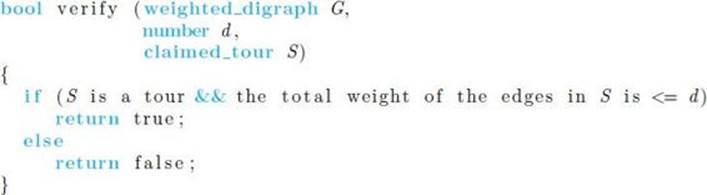
This algorithm first checks to see whether S is indeed a tour. If it is, the algorithm then adds the weights on the tour. If the sum of the weights is no greater than d, it returns “true.” This means that it has verified that yes, there is a tour with total weight no greater than d, and we know that the answer to the decision problem is “yes.” If S is not a tour or the sum of the weights exceeds d, the algorithm returns “false.” Returning false means only that this claimed tour is not a tour with total weight no greater than d. It does not mean that such a tour does not exist, because there might be a different tour with total weight no greater than d.

It is left as an exercise to implement the algorithm more concretely and show that it is polynomial-time. This means that, given a candidate tour, we can verify in polynomial time whether this candidate proves that the answer to our decision problem is “yes.” If the proposed tour turns out not to be a tour or to have total length greater than d (perhaps the person was bluffing), we have not proven that the answer must be “no” to our decision problem. Therefore, we are not talking about being able to verify that the answer to our decision problem is “no” in polynomial time.

It is this property of polynomial-time verifiability that is possessed by the problems in the set NP, which we define next. This does not mean that these problems can necessarily be solved in polynomial time. When we verify that a candidate tour has total weight no greater than d, we are not including the time it took to find that tour. We are only saying that the verification part takes polynomial time. To state the notion of polynomial-time verifiability more concretely, we introduce the concept of a nondeterministic algorithm. We can think of such an algorithm as being composed of the following two separate stages:

1. Guessing (Nondeterministic) Stage: Given an instance of a problem, this stage simply produces some string S. The string can be thought of as a guess at a solution to the instance. However, it could just be a string of nonsense.

2. Verification (Deterministic) Stage: The instance and the string S are the input to this stage. This stage then proceeds in an ordinary deterministic manner either (1) eventually halting with an output of “true,” which means that it has been verified that the answer for this instance is “yes,” (2) halting with an output of “false,” or (3) not halting at all (that is, going into an infinite loop). In these latter two cases, it has not been verified that the answer for this instance is “yes.” As we shall see, for our purposes these two cases are indistinguishable.

Function verify does the verification stage for the Traveling Salesperson Decision problem. Notice that it is an ordinary deterministic algorithm. It is the guessing stage that is nondeterministic. This stage is called nondeterministic because unique step-by-step instructions are not specified for it. Rather, in this stage, the machine is allowed to produce any string in an arbitrary matter. A “nondeterministic stage” is simply a definitional device for the purpose of obtaining the notion of polynomial-time verifiability. It is not a realistic method for solving a decision problem.

Even though we never actually use a nondeterministic algorithm to solve a problem, we say that a nondeterministic algorithm “solves” a decision problem if:

1. For any instance for which the answer is “yes,” there is some string S for which the verification stage returns “true.”

2. For any instance for which the answer is “no,” there is no string for which the verification stage returns “true.”

Figure 9.2 The tour [v₁, v₃, v₂, v₄, v₁] has total weight no greater than 15.

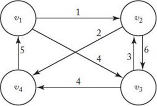
The following table shows the results of some input strings S to function verify when the instance is the graph in Figure 9.2 and d is 15.

The third input illustrates that S can just be a string of nonsense (as discussed previously).

In general, if the answer for a particular instance is “yes,” function verify returns “true” when one of the tours with total weight no greater than d is the input. Therefore, Criterion 1 for a nondeterministic algorithm is satisfied. On the other hand, function verify only returns “true” when a tour with total weight no greater than d is the input. Therefore, if the answer for an instance is “no,” function verify does not return “true” for any value of S, which means that Criterion 2 is satisfied. A nondeterministic algorithm that simply generates strings in the guessing state and calls function verify in the verification stage therefore “solves” the Traveling Salesperson Decision problem. Next we define what is meant by a polynomial-time nondeterministic algorithm.

Definition

A polynomial-time nondeterministic algorithm is a nondeterministic algorithm whose verification stage is a polynomial-time algorithm.

Now we can define the set NP.

Definition

NP is the set of all decision problems that can be solved by polynomial-time nondeterministic algorithms.

Note that NP stands for “nondeterministic polynomial.” For a decision problem to be in NP, there must be an algorithm that does the verification in polynomial time. Because this is the case for the Traveling Salesperson Decision problem, that problem is in NP. It must he stressed that this does not mean that we necessarily have a polynomial-time algorithm that solves the problem. Indeed, we do not presently have one for the Traveling Salesperson Decision problem. If the answer for a particular instance of that problem were “yes,” we might try all tours in the nondeterministic stage before trying one for which verify returns “true.” If there were an edge from every vertex to every other vertex, there would be (n − 1)! tours. Therefore, if all tours were tried, the answer would not be found in polynomial time. Furthermore, if the answer for an instance were “no,” solving the problem using this technique would absolutely require that all tours be tried. The purpose of introducing the concepts of nondeterministic algorithms and NP is to classify algorithms. There are usually better algorithms for actually solving a problem than an algorithm that generates and verifies strings. For example, the branch-and-bound algorithm for the Traveling Salesperson problem (Algorithm 6.3) does generate tours, but it avoids generating many of the tours by using a bounding function. Therefore, it is much better than an algorithm that blindly generates tours.

What other decision problems are in NP? In the exercises you are asked to establish that the other decision problems in Examples 9.2 to 9.5 are all in NP.

Furthermore, there are thousands of other problems that no one has been able to solve with polynomial-time algorithms but that have been proven to be in NP because polynomial-time nondeterministic algorithms have been developed for them. (Many of these problems appear in Garey and Johnson, 1979.) Finally, there is a large number of problems that are trivially in NP. That is, every problem in P is also in NP. This is trivially true because any problem in P can be solved by a polynomial-time algorithm. Therefore, we can merely generate any nonsense in the nondeterministic stage and run that polynomial-time algorithm in the deterministic stage. Because the algorithm solves the problem by answering “yes” or “no,” it verifies that the answer is “yes” (for an instance where it is “yes”) given any input string S.

What decision problems are not in NP? Curiously, the only decision problems that have been proven not to be in NP are the same ones that have been proven to be intractable. That is, the Halting problem, Presburger Arithmetic, and the other problems discussed in Section 9.3.2 have been proven not to be in NP. Again, we have found relatively few such problems.

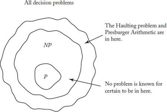
Figure 9.3 shows the set of all decision problems. Notice that in this figure NP contains P as a proper subset. However, this may not be the case. That is, no one has ever proven that there is a problem in NP that is not in P. Therefore, NP − P may be empty. Indeed, the question of whether Pequals NP is one of the most intriguing and important questions in computer science. This question is important, because, as we have already mentioned, most decision problems we have developed are in NP. Therefore, if P = NP, we would have polynomial-time algorithms for most known decision problems.

Figure 9.3 The set of all decision problems.

To show that P ≠ NP we would have to find a problem in NP that is not in P, whereas to show that P = NP we would have to find a polynomial-time algorithm for each problem in NP. Next we see that this latter task can be greatly simplified. That is, we show that it is necessary to find a polynomial-time algorithm for only one of a large class of problems. In spite of this great simplification, many researchers doubt that P equals NP.

• 9.4.2 NP-Complete Problems

The problems in Examples 9.2 to 9.5 may not all appear to have the same difficulty. For example, our dynamic programming algorithm (Algorithm 3.11) for the Traveling Salesperson problem is worst-case Θ(n²2ⁿ). On the other hand, our dynamic programming algorithm (in Section 4.4) for the 0-1 Knapsack problem is worst-case Θ(2ⁿ). Furthermore, the state space tree in the branch-and-bound algorithm (Algorithm 6.3) for the Traveling Salesperson problem has (n − 1)! leaves, whereas the one in the branch-and-bound algorithm (Algorithm 6.2) for the 0-1 Knapsack problem has only about 2ⁿ⁺¹ nodes. Finally, our dynamic programming algorithm for the 0-1 Knapsack problem is Θ(nW), which means that it is efficient as long as the capacity W of the sack is not extremely large. In light of all this, it seems that perhaps the 0-1 Knapsack problem is inherently easier than the Traveling Salesperson problem. We show that in spite of this, these two problems, the other problems in Examples 9.2 to 9.5, and thousands of other problems are all equivalent in the sense that if any one is in P, they all must be in P. Such problems are called NP-complete. To develop this result, we first describe a problem that is fundamental to the theory of NP-completeness—the problem of CNF-Satisfiability.

Example 9.6

CNF-Satisfiability Problem

A logical (Boolean) variable is a variable that can have one of two values: true or false. If x is a logical variable, is the negation of x. That is, x is true if and only if is false. A literal is a logical variable or the negation of a logical variable. A clause is a sequence of literals separated by the logical or operator (∨). A logical expression in conjunctive normal form (CNF) is a sequence of clauses separated by the logical and operator (∧). The following is an example of a logical expression in CNF:

The CNF-Satisfiability Decision problem is to determine, for a given logical expression in CNF, whether there is some truth assignment (some set of assignments of true and false to the variables) that makes the expression true.

Example 9.7

For the instance

the answer to CNF-Satisfiability is “yes,” because the assignments x₁ = true, x₂ = false, and x₃ = false make the expression true. For the instance

the answer to CNF-Satisfiability is “no,” because no assignment of truth values makes the expression true.

It is easy to write a polynomial-time algorithm that takes as input a logical expression in CNF and a set of truth assignments to the variables and verifies whether the expression is true for that assignment. Therefore, the problem is in NP. No one has ever found a polynomial-time algorithm for this problem, and no one has ever proven that it cannot be solved in polynomial time. So we do not know if it is in P. The remarkable thing about this problem is that in 1971, Stephen Cook published a paper proving that if CNF-Satisfiability is in P, then P = NP. (A variation of this theorem was published independently by L. A. Levin in 1973.) Before we can state the theorem rigorously, we need to develop a new concept—namely, the concept of polynomial-time reducibility.

Figure 9.4 Algorithm tran is a transformation algorithm that maps each instance x of decision problem A to an instance y of decision problem B. Together with the algorithm for decision problem B, it yields an algorithm for decision problem A.

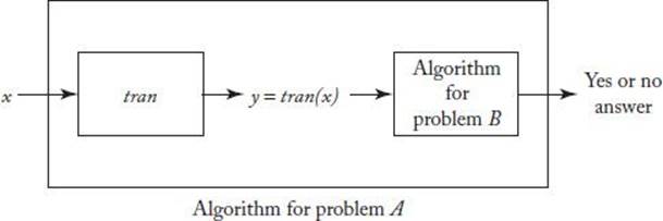
Suppose we want to solve decision problem A and we have an algorithm that solves decision problem B. Suppose further that we can write an algorithm that creates an instance y of problem B from every instance x of problem A such that an algorithm for problem B answers “yes” for y if and only if the answer to problem A is “yes” for x. Such an algorithm is called a transformation algorithm and is actually a function that maps every instance of problem A to an instance of problem B. We can denote it as follows:

The transformation algorithm combined with an algorithm for problem B yields an algorithm for problem A. Figure 9.4 illustrates this.

The following example has nothing to do with the theory of NP-completeness. We present it because it is a simple example of a transformation algorithm.

Example 9.8

A Transformation Algorithm

Let our first decision problem be: Given n logical variables, does at least one of them have the value “true”? Let our second decision problem be: Given n integers, is the largest of them positive? Let our transformation be:

where k₁ is 1 if x₁ is true and k_i is 0 if x_i is false. An algorithm for our second problem returns “yes” if and only if at least one k_i is 1, which is the case if and only if at least one x_i is true. Therefore, an algorithm for the second problem returns “yes” if and only if at least one x_i is true, which meansthat our transformation is successful, and we can solve the first problem using an algorithm for the second problem.

We have the following definition pertaining to the concepts just developed.

Definition

If there exists a polynomial-time transformation algorithm from decision problem A to decision problem B, problem A is polynomial-time many-one reducible to problem B. (Usually we just say that problem A reduces to problem B.) In symbols, we write

We say “many-one” because a transformation algorithm is a function that may map many instances of problem A to one instance of problem B. That is, it is a many-one function.

If the transformation algorithm is polynomial-time and we have a polynomial-time algorithm for problem B, intuitively it seems that the algorithm for problem A that results from combining the transformation algorithm and the algorithm for problem B must be a polynomial-time algorithm. For example, it is clear that the transformation algorithm in Example 9.8 is polynomial-time. Therefore, it seems that if we run that algorithm followed by some polynomial-time algorithm for the second problem, we are solving the first problem in polynomial time. The following theorem proves that this is so.

Theorem 9.1

If decision problem B is in P and

then decision problem A is in P.

Proof: Let p be a polynomial that bounds the time complexity of the polynomial-time transformation algorithm from problem A to problem B, and let q be a polynomial that bounds the time complexity of a polynomial-time algorithm for B. Suppose we have an instance of problem A that is of size n. Because at most there are p (n) steps in the transformation algorithm, and at worst that algorithm outputs a symbol at each step, the size of the instance of problem B produced by the transformation algorithm is at most p (n). When that instance is the input to the algorithm for problem B, this means that there are at most q [p (n)] steps. Therefore, the total amount of work required to transform the instance of problem A to an instance of problem B and then solve problem B to get the correct answer for problem A is at most

which is a polynomial in n.

Next we define NP-complete.

Definition

A problem B is called NP-complete if both of the following are true:

1. B is in NP.

2. For every other problem A in NP,

By Theorem 9.1, if we could show that any NP-complete problem is in P, we could conclude that P = NP. In 1971 Stephen Cook managed to find a problem that is NP-complete. The following theorem states his result.

Theorem 9.2

(Cook’s Theorem) CNF-Satisfiability is NP-complete.

Proof: The proof can be found in Cook (1971) and in Garey and Johnson (1979).

Although we do not prove Cook’s theorem here, we mention that the proof does not consist of reducing every problem in NP individually to CNF-Satisfiability. If this were the case, whenever a new problem in NP was discovered, it would be necessary to add its reduction to the proof. Rather, the proof exploits common properties of problems in NP to show that any problem in this set must reduce to CNF-Satisfiability.

Once this ground-breaking theorem was proven, many other problems were proven to be NP-complete. These proofs rely on the following theorem.

Theorem 9.3

A problem C is NP-complete if both of the following are true:

1. C is in NP.

2. For some other NP-complete problem B,

Proof: Because B is NP-complete, for any problem A in NP, A ∝ B. It is not hard to see that reducibility is transitive. Therefore, A ∝ C. Because C is in NP, we can conclude that C is NP-complete.

By Cook’s theorem and Theorem 9.3, we can show that a problem is NP-complete by showing that it is in NP and that CNF-Satisfiability reduces to it. These reductions are typically much more complex than the one given in Example 9.7. We give one such reduction next.

Example 9.9

We show that the Clique Decision problem is NP-complete. It is left as an exercise to show it is in NP by writing a polynomial-time verification algorithm for this problem. Therefore, we need only show that

to conclude that the problem is NP-complete. First recall that a clique in an undirected graph is a subset of vertices such that each vertex in the subset is adjacent to all the other vertices in the subset, and that the Clique Decision problem is to determine for a graph and a positive integer k whether the graph has a clique containing at least k vertices. Let

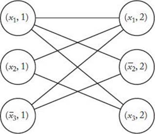
be a logical expression in CNF, where each C_i is a clause of B, and let x₁, x₂, …, x_n be the variables in B. Transform B to a graph G = (V, E), as follows:

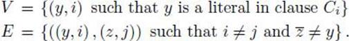
A sample construction of G is shown in Figure 9.5. It is left as an exercise to show that this transformation is polynomial-time. Therefore, we need only show that B is CNF-Satisfiable if and only if G has a clique of size at least k. We do this next.

1. Show that if B is CNF-Satisfiable, G has a clique of size at least k: If B is CNF-Satisfiable, there are truth assignments for x₁, x₂, …, x_n such that each clause is true with these assignments. This means that with these assignments there is at least one literal in each C_i that is true. Pick one such literal from each C_i. Then let

Clearly, V′ forms a clique in G of size k.

Figure 9.5 The graph G in Example 9.9 when B = (x₁ ∨ x₂ ∨ x₃) ∧ (x₁ ∨ ₂ ∨ x₃).

2. Show that if G has a clique of size at least k, B is CNF-Satisfiable: Because there cannot be an edge from a vertex (y, i) to a vertex (z, i), the indices in the vertices in a clique must all be different. Because there are only k different indices, this means that a clique can have at most k vertices. So ifG has a clique (V′, E′) of size at least k, the number of vertices in V′ must be exactly k. Therefore, if we set

S contains k literals. Furthermore, S contains a literal from each of the k clauses, because there is no edge connecting (y, i) and (z, i) for any literals y and z and index i. Finally, S cannot contain both a literal y and its complement y, because there is no edge connecting (y, i) and (y, j) for any i andj. Therefore, if we set

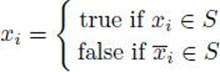
and assign arbitrary truth values to variables not in S, all clauses in B are true. Therefore, B is CNF-Satisfiable.

Recall the Hamiltonian Circuits problem from Section 5.6. The Hamiltonian Circuits Decision problem is to determine whether a connected, undirected graph has at least one tour (a path that starts at one vertex, visits each vertex in the graph once, and ends up at the starting vertex). It is possible to show that

The reduction is even more tedious than the one given in the previous example and can be found in Horowitz and Sahni (1978). It is left as an exercise to write a polynomial-time verification algorithm for this problem. Therefore, we can conclude that the Hamiltonian Circuits Decision problem isNP-complete.

Now that we know that the Clique Decision problem and the Hamiltonian Circuits Decision problem are NP-complete, we can show that some other problem in NP is NP-complete by showing that the Clique Decision problem or the Hamiltonian Circuits Decision problem reduces to that problem (by Theorem 9.3). That is, we do not need to return to CNF-Satisfiability for each proof of NP-completeness. More sample reductions follow.

Example 9.10

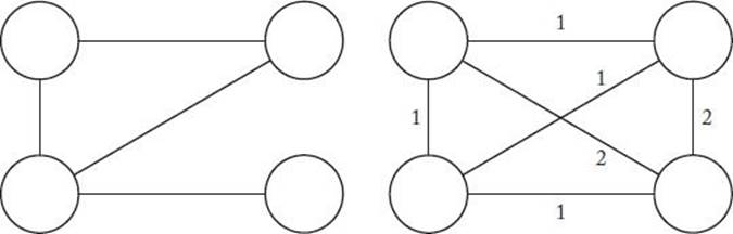
Consider a variant of the Traveling Salesperson Decision problem in which the graph is undirected. That is, given a weighted, undirected graph and a positive number d, determine whether there is an undirected tour having total weight no greater than d. Clearly, the polynomial-time verification algorithm given earlier for the usual Traveling Salesperson problem also works for this problem. Therefore the problem is in NP, and we need only show that some NP-complete problem reduces to it to conclude that it is NP-complete. We show that

Transform an instance (V, E) of the Hamiltonian Circuits Decision problem to the instance (V, E′) of the Traveling Salesperson (Undirected) Decision problem that has the same set of vertices V, has an edge between every pair of vertices, and has the following weights:

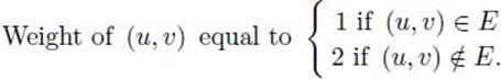
An example of this transformation is shown in Figure 9.6. Clearly, (V, E) has a Hamiltonian Circuit if and only if (V, E′) has a tour with total weight no more than n, where n is the number of vertices in V. It is left as an exercise to complete this example by showing that the transformation is polynomial-time.

Figure 9.6 The transformation algorithm in Example 9.10 maps the undirected graph on the left to the weighted, undirected graph on the right.

Example 9.11

We have already written a polynomial-time verification algorithm for the usual Traveling Salesperson Decision problem. Therefore, this problem is in NP, and we can show that it is NP-complete by showing that

Transform an instance (V, E) of the Traveling Salesperson (Undirected) Decision problem to the instance (V, E′) of the Traveling Salesperson problem that has the same set of vertices V and has the edges ⟨u, v⟩ and ⟨v, u⟩ both in E′ whenever (u, v) is in E. The directed weights of ⟨u, v⟩ and ⟨v, u⟩are the same as the undirected weight of (u, v). Clearly, (V, E) has an undirected tour with total weight no greater than d if and only if (V, E′) has a directed tour with total weight no greater than d. It is left as an exercise to complete this example by showing that the transformation is polynomial-time.

As mentioned previously, thousands of problems, including the other problems in Examples 9.2 to 9.5, have been shown to be NP-complete using reductions like those just given. Garey and Johnson (1979) contains many sample reductions and lists over 300 NP-complete problems.

The State of NP

Figure 9.3 shows P as a proper subset of NP, but, as mentioned previously, they may be the same set. How does the set of NP-complete problems fit into the picture? First, by definition, it is a subset of NP. Therefore, Presburger Arithmetic, the Halting problem, and any other decision problems that are not in NP are not NP-complete.

A decision problem that is in NP and is not NP-complete is the trivial decision problem that answers “yes” for all instances (or answers “no” for all instances). This problem is not NP-complete because it is not possible to transform a nontrivial decision problem to it.

If P = NP, the situation is as depicted on the left in Figure 9.7. If P ≠ NP, the situation is as depicted on the right in that figure. That is, if P ≠ NP, then

where NP-complete denotes the set of all NP-complete problems. This is so because if some problem in P were NP-complete, Theorem 9.1 would imply that we could solve any problem in NP in polynomial time.

Figure 9.7 The set NP is either as depicted on the left or as depicted on the right.

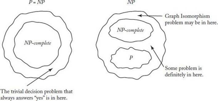
Notice that Figure 9.7 (on the right) says that the Graph Isomorphism problem may be in

This problem concerns graph isomorphism, which is defined as follows. Two graphs (undirected or directed) G = (V, E) and G′ = (V′, E′) are called isomorphic if there is a one-to-one function f from V onto V′ such that for every v₁ and v₂ in V, the edge (u, v) is in E if and only if the edge (f(u) , f(v)) is in E′. The Graph Isomorphism problem is as follows:

Example 9.12

Graph Isomorphism Problem

Given two graphs G = (V, E) and G′ = (V′, E′), are they isomorphic?

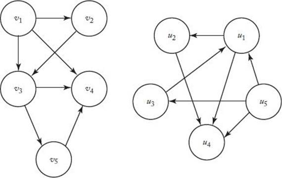
The directed graphs in Figure 9.8 are isomorphic owing to the function

It is left as an exercise to write a polynomial-time verification algorithm for the Graph Isomorphism problem, and thereby show it is in NP. A straightforward algorithm for this problem is to check all n! one-to-one onto mappings, where n is the number of vertices. This algorithm has worse than exponential time complexity. No one has ever found a polynomial-time algorithm for this problem; yet no one has ever proven it is NP-complete. Therefore, we do not know whether it is in P and we do not know whether it is NP-complete.

No one has been able to prove that there is a problem in NP that is neither in P nor NP-complete (such a proof would automatically prove that P ≠ NP). However, it has been proved that, if P ≠ NP, such a problem must exist. This result, which is stated on the right in Figure 9.7, is formalized in the following theorem.

Figure 9.8 These graphs are isomorphic.

Theorem 9.4

If P ≠ NP, the set

is not empty.

Proof: The proof follows from a more general result that can be found in Ladner (1975).

Complementary Problems

Notice the similarity between the following two problems.

Example 9.13

Primes Problem

Given a positive integer n, is n a prime number?

Example 9.14

Composite Numbers Problem

Given a positive integer n, are there integers m > 1 and k > 1 such that n = mk?

The Primes problem is the one solved by the algorithm at the beginning of Section 9.2. It is the complementary problem to the Composite Numbers problem. In general, the complementary problem to a decision problem is the problem that answers “yes” whenever the original problem answers “no” and answers “no” whenever the original problem answers “yes.” Another example of a complementary problem follows.

Example 9.15

Complementary Traveling Salesperson Decision Problem

Given a weighted graph, and a positive number d, is there no tour with total weight no greater than d?

Clearly, if we found an ordinary deterministic polynomial-time algorithm for a problem, we would have a deterministic polynomial-time algorithm for its complementary problem. For example, if we could determine in polynomial-time whether a number was composite, we would also be determining whether it was prime. However, finding a polynomial-time non-deterministic algorithm for a problem does not automatically produce a polynomial-time nondeterministic algorithm for its complementary. That is, showing that one is in NP does not automatically show that the other is inNP. In the case of the Complementary Traveling Salesperson problem, the algorithm would have to be able to verify in polynomial time that no tour with weight no greater than d exists. This is substantially more complex than verifying that a tour has weight no greater than d. No one has ever found a polynomial-time verification algorithm for the Complementary Traveling Salesperson Decision Problem. Indeed, no one has ever shown that the complementary problem to any known NP-complete problems is in NP. On the other hand, no one has ever proven that some problem is in NPwhereas its complementary problem is not in NP. The following result has been obtained.

Theorem 9.5

If the complementary problem to any NP-complete problem is in NP, the complementary problem to every problem in NP is in NP.

Proof: The proof can be found in Garey and Johnson (1979).

Let’s discuss the Graph Isomorphism and Primes problem further. As mentioned in the previous subsection, no one has ever found a polynomial-time algorithm for the Graph Isomorphism problem, yet no one has proven that it is NP-complete. Until recently, the same was true of the Primes problem. However, in 2002 Agrawal et al. developed a polynomial-time algorithm for the Primes problem. We present that algorithm in Section 10.6. Before than, in 1975 Pratt had shown the Primes problem to be in NP, and it straightforward to show its complementary problem (the Composite Numbers problem) is in NP. Similarly, the Linear Programming problem and its complementary problem were both shown to be in NP before Chachian (1979) developed a polynomial-time algorithm for it. On the other hand, no one has been able to show the complementary problem to the Graph Isomorphism problem is in NP. Given these results, it seems more likely that the Graph Isomorphism problem will be shown to be NP-complete than that we will find a polynomial-time algorithm for it. On the other hand, it may be in the set NP − (P ∪ NP-complete).

• 9.4.3 NP-Hard, NP-Easy, and NP-Equivalent Problems

So far we have discussed only decision problems. Next we extend our results to problems in general. Recall that Theorem 9.1 implies that if decision problem A is polynomial-time many-one reducible to problem B, then we could solve problem A in polynomial time using a polynomial-time algorithm for problem B. We generalize this notion to nondecision problems with the following definition.

Definition

If problem A can be solved in polynomial time using a hypothetical polynomial time algorithm for problem B, then problem A is polynomial-time Turing reducible to problem B. (Usually we just say A Turing reduces to B.) In symbols, we write

This definition does not require that a polynomial-time algorithm for problem B exist. It only says that if one did exist, problem A would also be solvable in polynomial time. Clearly, if A and B are both decision problems, then

Next we extend the notion of NP-completeness to nondecision problems.

Definition

A problem B is called NP-hard if, for some NP-complete problem A,

It is not hard to see that Turing reductions are transitive. Therefore, all problems in NP reduce to any NP-hard problem. This means that if a polynomial-time algorithm exists for any NP-hard problem, then P = NP.

What problems are NP-hard? Clearly, every NP-complete problem is NP-hard. Therefore, we ask instead what nondecision problems are NP-hard. Earlier we noted that if we could find a polynomial-time algorithm for an optimization problem, we would automatically have a polynomial-time algorithm for the corresponding decision problem. Therefore, the optimization problem corresponding to any NP-complete problem is NP-hard. The following example formally uses the definition of Turing reducibility to show this result for the Traveling Salesperson problem.

Example 9.16

The Traveling Salesperson Optimization Problem Is NP -hard

Suppose we had a hypothetical polynomial-time algorithm for the Traveling Salesperson Optimization problem. Let the instance of the Traveling Salesperson Decision problem containing the graph G and positive integer d be given. Apply the hypothetical algorithm to the graph G to obtain the optimal solution mindist. Then our answer for the instance of the decision problem would be “no” if d ≤ mindist and “yes” otherwise. Clearly, the hypothetical polynomial-time algorithm for the optimization problem, along with this extra step, gives the answer to the decision problem in polynomial time. Therefore,

What problems are not NP-hard? We do not know if there is any such problem. Indeed, if we were to prove that some problem was not NP-hard, we would be proving that P ≠ NP. The reason is that if P = NP, then each problem in NP would be solvable by a polynomial-time algorithm. Therefore, we could solve each problem in NP, using a hypothetical polynomial-time algorithm for any problem B, by simply calling the polynomial-time algorithm for each problem. We don’t even need the hypothetical algorithm for problem B. Therefore, all problems would be NP-hard.

On the other hand, any problem for which we have found a polynomial-time algorithm may not be NP-hard. Indeed, if we were to prove that some problem for which we had a polynomial-time algorithm was NP-hard, we would be proving that P = NP. The reason is that we would then have an actual rather than a hypothetical polynomial-time algorithm for some NP-hard problem. Therefore, we could solve each problem in NP in polynomial-time using the Turing reduction from the problem to the NP-hard problem.

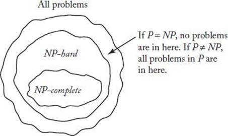
Figure 9.9 illustrates how the set of NP-hard problems fits into the set of all problems.

Figure 9.9 The set of all problems.

If a problem is NP-hard, it is at least as hard (in terms of our hopes of finding a polynomial-time algorithm) as the NP-complete problems. For example, the Traveling Sales Optimization problem is at least as hard as the NP-complete problems. However, is the reverse necessarily true? That is, are the NP-complete problems at least as hard as the Traveling Salesperson Optimization problem? NP-hardness does not imply this. We need another definition.

Definition

A problem A is called NP-easy if, for some problem B in NP,

Clearly, if P = NP, then a polynomial-time algorithm exists for all NP-easy problems. Notice that our definition of NP-easy is not exactly symmetrical with our definition of NP-hard. It is left as an exercise to show that a problem is NP-easy if and only if it reduces to an NP-complete problem.

What problems are NP-easy? Obviously, the problems in P, the problems in NP, and nondecision problems for which we have found polynomial-time algorithms are all NP-easy. The optimization problem, corresponding to an NP-complete decision problem, can usually be shown to be NP-easy. However, it is not trivial to do this, as the following example illustrates.

Example 9.17

The Traveling Salesperson Optimization problem is NP-easy. To establish this result, we introduce the following problem.

Traveling Salesperson Extension Decision Problem

Let an instance of the Traveling Salesperson Decision problem be given, where the number of vertices in the graph is n and the integer is d. Furthermore, let a partial tour T consisting of m distinct vertices be given. The problem is to determine whether T can be extended to a complete tour having total weight no greater than d. The parameters for this problem are the same as those for the Traveling Salesperson Decision problem plus the partial tour T.

It is not hard to show that the Traveling Salesperson Extension Decision problem is in NP. Therefore, in order to obtain our desired result, we need only show that

To that end, let polyalg be a hypothetical polynomial-time algorithm for the Traveling Salesperson Extension Decision problem. The inputs to polyalg are a graph, a partial tour, and a distance. Let an instance G of size n of the Traveling Salesperson Optimization problem be given. Let the vertices in the instance be

and set

If mindist is the total weight of the edges in an optimal tour, then

Because any vertex can be the first vertex on our tour, we can make v₁ the first vertex. Consider the following call:

The partial tour that is the input to this call is simply [v₁], which is the partial tour before we ever leave v₁. The smallest value of d for which this call could return “true” is d = dmin, and if there is a tour, the call will definitely return “true” if d = dmax. If it returns “false” for d = dmax, then mindist =∞. Otherwise, using a binary search, we can determine the smallest value of d for which polyalg returns “true” when G and [v₁] are the inputs. That value is mindist. This means that we can compute mindist in at most about lg(dmax) calls to polyalg, which means that we can compute mindist in polynomial time.

Once we know the value of mindist, we use polyalg to construct an optimal tour in polynomial time, as follows. If mindist = ∞, there are no tours, and we are done. Otherwise, say that a partial tour is extendible if it can be extended to a tour having total weight equal to mindist. Clearly, [v₁] is extendible. Because [v₁] is extendible, there must be at least one v_i such that [v₁, v_i] is extendible. We can determine such a v_i by calling polyalg at most n − 2 times, as follows:

where 2 ≤ i ≤ n − 1. We stop when we find an extendible tour or when i reaches n − 1. We need not check the last vertex, because, if the others all fail, the last vertex must be extendible.

In general, given an extendible partial tour containing m vertices, we can find an extendible partial tour containing m + 1 vertices with at most n − m − 1 calls to polyalg. So we can build an optimal tour with at most the following number of calls to polyalg:

This means that we can also construct an optimal tour in polynomial time, and we have a polynomial-time Turing reduction.

Similar proofs have been established for the other problems in Examples 9.2 to 9.5 and for the optimization problems corresponding to most NP-complete decision problems. We have the following definition concerning such problems.

Definition

A problem is called NP-equivalent if it is both NP-hard and NP-easy.

Clearly, P = NP if and only if polynomial-time algorithms exist for all NP-equivalent problems.

We see that originally restricting our theory to decision problems causes no substantial loss in generality, because we can usually show that the optimization problem, corresponding to an NP-complete decision problem, is NP-equivalent. This means that finding a polynomial-time algorithm for the optimization problem is equivalent to finding one for the decision problem.

Our goal has been to provide a facile introduction to the theory of NP. For a more thorough introduction, you are referred to the text we have referenced several times—namely, Garey and Johnson (1979). Although that text is quite old, it is still one of the best comprehensive introductions to theNP theory. Another good introductory text is Papadimitriou (1994).

9.5 Handling NP-Hard Problems

In the absence of polynomial-time algorithms for problems known to be NP-hard, what can we do about solving such problems? We presented one way in Chapters 5 and 6. The backtracking and branch-and-bound algorithms for these problems are all worst-case nonpolynomial-time. However, they are often efficient for many large instances. Therefore, for a particular large instance of interest, a backtracking or branch-and-bound algorithm may suffice. Recall from Section 5.3 that the Monte Carlo technique can be used to estimate whether a given algorithm would be efficient for a particular instance. If the estimate shows that it probably would be, we can try using the algorithm to solve that instance.

Another approach is to find an algorithm that is efficient for a subclass of instances of an NP-hard problem. For example, the problem of probabilistic inference in a Bayesian network, discussed in Section 6.3, is NP-hard. In general, a Bayesian network consists of a directed acyclic graph and a probability distribution. Polynomial-time algorithms have been found for the subclass of instances in which the graph is singly connected. A directed, acyclic graph is singly connected if there is no more than one path from any vertex to any other vertex. Pearl (1988) and Neapolitan (1990, 2003) discuss these algorithms.

A third approach, investigated here, is to develop approximation algorithms. An approximation algorithm for an NP-hard optimization problem is an algorithm that is not guaranteed to give optimal solutions, but rather yields solutions that are reasonably close to optimal. Often we can obtain a bound that gives a guarantee as to how close a solution is to being optimal. For example, we derive an approximation algorithm that gives a solution, which we will call minapprox, to a variant of the Traveling Salesperson Optimization problem. We show that

where mindist is the optimal solution. This does not mean that minapprox is always almost twice mindist. For many instances, it may be much closer or even equal to mindist. Rather, this means that we are guaranteed that minapprox will never be as great as twice mindist. We develop this algorithm and an improvement on it next. Then we further illustrate approximation algorithms by deriving one for another problem.

• 9.5.1 An Approximation Algorithm for the Traveling Salesperson Problem

Our algorithm will be for the following variant of the problem.

Example 9.18

Traveling Salesperson Problem with Triangular Inequality

Let a weighted, undirected graph G = (V, E) be given such that

1. There is an edge connecting every two distinct vertices.

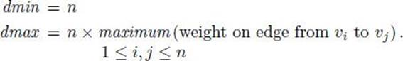
2. If W (u, v) denotes the weight on the edge connecting vertex u to vertex v, then, for every other vertex y,

The second condition, called the triangular inequality, is depicted in Figure 9.10. It is satisfied if the weights represent actual distances (“as the crow flies”) between cities. Recall that weight and distance terminology are used interchangeably for weighted graphs. The first condition implies that there is a two-way road connecting every city to every other city.

The problem is to find the shortest path (optimal tour) starting and ending at the same vertex and visiting each other vertex exactly once. It can be shown that this variant of the problem is also NP-hard.

Notice that the graph in this variant of the problem is undirected. If we remove any edge from an optimal tour for such a graph, we have a spanning tree for the graph. Therefore, the total weight of a minimum spanning tree must be less than the total weight of an optimal tour. We can use Algorithm 4.1 or 4.2 to obtain a minimum spanning tree in polynomial time. By going twice around the spanning tree, we can convert it to a path that visits every city. This is illustrated in Figure 9.11. A graph is depicted in Figure 9.11(a), a minimum spanning tree for the graph in Figure 9.11(b), and the path obtained by going twice around the tree in Figure 9.11(c). As the figure shows, the resulting path may visit some vertices more than once. We can convert the path to one that does not do this by taking “shortcuts.” That is, we traverse the path, starting at some arbitrary vertex, and visit each unvisited vertex in sequence. When there is more than one unvisited vertex adjacent to the current vertex in the tree, we simply visit the closest one. If the only vertices adjacent to the current vertex have already been visited, we bypass them by means of a shortcut to the next unvisited vertex. The triangular inequality guarantees that the shortcut will not lengthen the path. Figure 9.11(d) shows the tour obtained using this technique. In that figure, we started with the bottom vertex on the left. Notice that the tour obtained is not optimal. However, if we start with the top left vertex, we obtain an optimal tour.

Figure 9.10 The triangular inequality implies that the “distance” from u to v is no greater than the “distance” from u to y plus the “distance” from y to v.

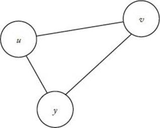
Figure 9.11 Obtaining an approximation to an optimal tour from a minimum spanning tree.

The method just outlined can be summarized in the following steps:

1. Determine a minimum spanning tree.

2. Create a path that visits every city by going twice around the tree.

3. Create a path that does not visit any vertex twice (that is, a tour) by taking shortcuts.

In general, the tour obtained using this method is not necessarily optimal regardless of the starting vertex. However, the following theorem gives us a guarantee as to how close the tour is to being optimal.

Theorem 9.6

Let mindist be the total weight of an optimal tour and minapprox be the total weight of the tour obtained using the method just described. Then

Proof: As we have already discussed, the total weight of a minimum spanning tree is less than mindist. Because the total weight of minapprox is no more than the total weight of two minimum spanning trees, the theorem follows.

It is possible to create instances that show that minapprox can be made arbitrarily close to 2 × mindist. Therefore, in general, the bound obtained in Theorem 9.6 is the best we can do.

We can obtain an even better approximation algorithm for this problem as follows. First obtain a minimum spanning tree as done above. Then consider the set V′ of all vertices that touch an odd number of edges. It is not hard to show that there must be an even number of such vertices. Pair up the vertices in V′ so that each vertex is paired with precisely one other vertex. Such a creation of vertex pairs is called a matching for V′. Add the edge connecting each vertex pair to the spanning tree. Because each vertex then has an even number of edges touching it, the resultant path visits every city. Furthermore, the total number of edges in this path is no greater than (and often is less than) the total number that would he obtained by simply going twice around the tree. Figure 9.12(a) shows a minimum spanning tree, and Figure 9.12(b) shows the path obtained from that tree with one possible matching. Figure 9.12(c) shows a tour obtained after shortcuts are taken.

Figure 9.12 A tour obtained using a matching.

A minimal weight matching for V′ is one such that the total weight of the edges obtained from the matching is minimal. Lawler (1976) shows how to obtain a minimal weight matching in polynomial time. We therefore can approximately solve the variant of the Traveling Salesperson problem given in Example 9.17 in polynomial-time using the following steps:

1. Obtain a minimum spanning tree.

2. Obtain a minimal weight matching of the vertices in V′, where V′ is the set of vertices in the spanning tree that touch an odd number of edges.

3. Create a path that visits every vertex by adding the edges connecting matched vertices to the tree.

4. Obtain a path that does not visit any vertex twice (that is, a tour) by taking shortcuts.

Figure 9.11 illustrates these steps without showing any actual weights. The following theorem shows that this method gives a better bound than the first method presented in this section.

Theorem 9.7

Let mindist be the total weight of an optimal tour and minapprox2 be the total weight of the tour obtained using the method of minimal weight matching. Then

Proof: Let V′ be the set of all vertices that touch an odd number of edges. Convert an optimal tour to a path connecting only the vertices in V′ by bypassing vertices not in V′. By the triangular inequality, the total weight of this path can be no greater than mindist. Furthermore, this path provides us with two matchings for the vertices in V′, as follows. Choose an arbitrary vertex in V′ and match it with the vertex on one side of it in the path. Then continue to match adjacent vertices in pairs going in this same direction. This is one match. Next match the initial vertex with the vertex on the other side of it in the path, and continue to match adjacent vertices going in the other direction. This is a second match. Because the edges in the two matches comprise all the edges in the path, the sum of the total weights of the two matches is equal to the weight of the path. Therefore, at least one of the matches has total weight no greater than half the weight of the path. Because the weight of this path is no greater than mindist, and because the weight of any matching is at least as great as the weight of a minimal weight matching, we have

where minmatch is the weight of a minimal weight matching. Recall that the weight of a minimum spanning tree is less than mindist. Because the edges obtained in Step 3 of the method of minimal weight matching consist of the edges in a spanning tree and the edges obtained from a minimal matching, the total weight of those edges is less than 1.5 × mindist. The theorem now follows, because the total weight of the edges in the final tour obtained in Step 4 is no greater than the weight of those obtained in Step 3.

It is possible to create instances for which the approximation can be made arbitrarily close to 1.5 × mindist. Therefore, in general, there is no better bound for this algorithm than the one obtained in Theorem 9.7.

Recall that our salesperson Nancy was last trying to find an optimal tour for her 40-city sales territory using a branch-and-bound algorithm (Algorithm 6.3) for the Traveling Salesperson problem. Because that algorithm is worst-case nonpolynomial-time, it may take many years to solve her particular instance. If the distances between Nancy’s cities satisfy the assumptions in the Traveling Salesperson with Triangular Inequality problem, she finally has an alternative that is sure to work. That is, she can use the method of minimal weight matching to obtain a good approximation to an optimal tour in polynomial time.

• 9.5.2 An Approximation Algorithm for the Bin-Packing Problem

We introduce the following new problem.

Example 9.19

Bin-Packing Problem

Let n items with sizes

be given, and suppose we are to pack the items in bins, where each bin has a capacity of 1. The problem is to determine the minimum number of bins necessary to pack all the items.

This problem has been shown to be NP-hard. A very simple approximation algorithm for this problem is called “first fit.” The first-fit strategy places an item in the first bin in which it fits. If it does not fit in a bin, a new bin is started. Another good idea is to pack the items in nonincreasing order.

Therefore, our strategy is called nonincreasing first fit. It can be described by the following high-level algorithm:

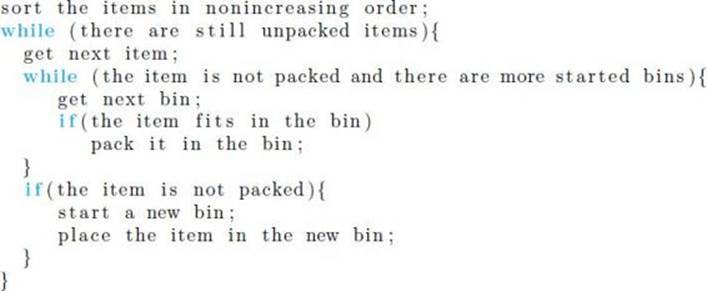
Figure 9.13 shows a result of applying this algorithm. Notice that it consists of a greedy algorithm within a greedy algorithm. That is, we greedily grab items, and for each item we greedily grab bins. It is left as an exercise to write a detailed version of this algorithm and show that it is Θ(n²). Notice that the solution in Figure 9.12 is not optimal. We could fit the items in only three bins if we placed the size 0.5 item, the size 0.3 item, and one of the size 0.2 items in the second bin, and placed the two size 0.4 items and one of the size 0.2 items in the third bin.

Next we obtain a bound for how close the approximate solution is to an optimal solution. The bound is obtained in Theorem 9.8. The proof of that theorem requires the following two lemmas.

Lemma 9.1

Let opt be the optimal number of bins for a given instance of the Bin-Packing problem. Any item that is placed by the nonincreasing first-fit strategy in an extra bin (that is, in a bin with index greater than opt) has size at most equal to 1/3.

Figure 9.13 A result of applying nonincreasing first fit.

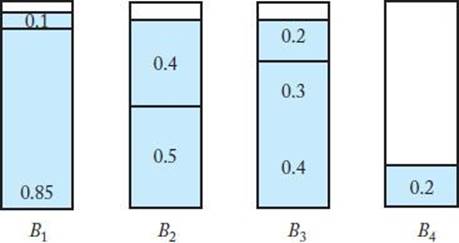
Proof: Let i be the index of the first item placed in bin opt + 1. Because the items are sorted in nonincreasing order, it suffices to show that

Suppose by way of contradiction that s_i > 1/3. Then

which means that all those bins with indices no greater than opt contain at most two items each. If every one of those bins contained two items, in an optimal solution there would have to be two of the first i − 1 items in every bin. But because their sizes are all greater than , there would be no room for s_i in one of the bins. Therefore, at least one bin with index no greater than opt contains only one item. If every bin with index no greater than opt contained only one item, no two of them could fit in a bin together and the ith item could not fit with any one of them (otherwise, our algorithm would have placed it with one of them). But then an optimal solution would require more than opt bins. Therefore, at least one bin with index no greater than opt contains two items.

We show that there is some j such that 0 < j < opt for which the first j bins contain one item each and the remaining opt − j bins contain two items each. If this were not the case, there would be bins B_k and B_m with k < m such that B_k contained two items and B_m contained one item. However, because the items are packed in nonincreasing order, the item packed in B_m would be no larger than the first item packed in B_k, and s_i would be no larger than the second item packed in B_k. Therefore, the sum of the sizes of the item in B_m and s_i would be no greater than the sum of the sizes of the two items in B_k, which means that s_i would fit in B_m. Therefore, the conjecture above (concerning j) must be true, and the bins appear as depicted in Figure 9.14.

Let an optimal solution be given. In such a solution, the first j items are in j distinct bins, because if any of them could fit together in a bin, our method would have put them together. Furthermore, items

are in the remaining opt−j bins, because none of them can fit with the first j items. Because our algorithm places two of each of these items in opt − j bins, there must be 2 × (opt − j) of these items. Because we assumed that the size of each of these items is greater than 1/3, there cannot be three of them in any of one of the remaining opt − j bins, which means that there must be exactly two items in each of these bins. Because we assumed that the size of s_i is also greater than 1/3, it cannot fit in the opt − j bins containing two items each. Furthermore, it cannot fit in one of the bins containing one of the first j items, because if it could fit with one of those items our algorithm would have placed it with that item. Because we assumed that this is an optimal solution, s_i must be in one of the bins, which means that we have a contradiction, and our lemma is proven.

Figure 9.14 If s_i > 1/3, our algorithm would pack the bins like this.

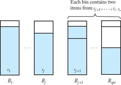
Lemma 9.2

Let opt be the optimal number of bins for an instance of the Bin-Packaging problem. The number of items placed by the nonincreasing first fit strategy in extra bins is at most opt − 1.

Proof: Because all the objects fit in opt bins,

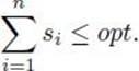
Suppose by way of contradiction that our approximation algorithm does put opt items into extra bins. Let z₁, z₂, … , z_opt be the sizes of those items, and, for 1 ≤ i ≤ opt, let tot_i be the total size that our algorithm puts in bin B_i. It must be true that

because otherwise the item of size z_i could have been put in B_i. We therefore have

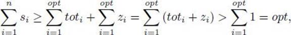
which contradicts what we showed at the beginning of the proof. This contradiction proves the lemma.

Theorem 9.8

Let opt be the optimal number of bins for an instance of the Bin-Packing problem, and let approx be the number of bins used by the nonincreasing first fit algorithm. Then

Proof: By Lemmas 9.1 and 9.2, the nonincreasing first-fit algorithm puts at most opt − 1 items, each of size at most in extra bins. Therefore, the number of extra bins is at most

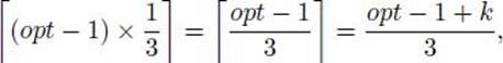
where k = 0, 1, or 2. Taking the largest possible value of k, we conclude that the number of extra bins is less than or equal to (opt + 1)/3, which means that

and therefore

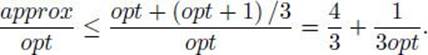
This ratio is maximized if opt = 1. However, when opt = 1, our approximation algorithm uses only one bin and therefore is optimal. This means that we can take opt = 2 to maximize the ratio and conclude that

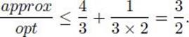
It is possible to create instances of arbitrarily large size for which the ratio is exactly 3/2. Therefore, in general, we cannot improve on the bound obtained in Theorem 9.8.

One way to gain further insight into the quality of an approximation algorithm is to run empirical tests comparing the solutions obtained from the approximation with the optimal solutions. Our approximation algorithm for the Bin-Packing problem has been extensively tested for large values of n. You may wonder how this is possible when we have no polynomial-time algorithm that guarantees an optimal solution, which means that we cannot determine an optimal solution for a large value of n in a tolerable amount of time. Indeed, if we had such an algorithm we would not bother with an approximation algorithm in the first place. The answer to this paradox is that in the case of the Bin-Packing problem we do not need to actually compute optimal solutions to gain insight into the quality of the approximations. Instead, we can compute the amount of unused space (the empty space) in the bins used by the approximation algorithm. The number of extra bins used by that algorithm can be no more than the amount of unused space. This is so because we can rearrange the items in our approximate solution so that they are in an optimal number of bins, leaving the extra bins empty. The amount of unused space in this optimal solution plus the total space in the extra bins is equal to the amount of unused space in our approximate solution. Therefore, because the total space in the extra bins equals the number of extra bins, the number of extra bins can be no greater than the amount of unused space in our approximate solution.

In an empirical study in which the input size was 128,000 and the item sizes were uniformly distributed between 0 and 1, our approximation algorithm used on the average about 64,000 bins, and on the average had about 100 units of unused space. This means that on the average the number of extra bins is bounded by 100 in the instances in this study. Theorem 9.8 implies, for an approximate solution of 64,000, that

which means opt ≥ 42, 666, and that the number of extra bins is no greater than 21,334. We see that the empirical study indicates that on the average, our algorithm performs much better than the upper bound.

For any particular instance of interest, we can compute the amount of unused space in the solution produced by the approximation algorithm. In this way we can determine how well the algorithm performs for that instance.

For more examples of approximation algorithms, you are again referred to Garey and Johnson (1979).

EXERCISES

Sections 9.1 to 9.3

1. List three problems that have polynomial-time algorithms. Justify your answer.

2. Give a problem and two encoding schemes for its input. Express its performance using your encoding schemes.

3. Show that a graph problem using the number of vertices as the measure of the size of an instance is polynomially equivalent to one using the number of edges as the measure of the size of an instance.

4. In which of the three general categories discussed in Section 9.3 does the problem of computing the nth Fibonacci term belong? Justify your answer.

5. A graph has an Euler Circuit if and only if (a) the graph is connected and (b) the degree of every vertex is even. Find a lower bound for the time complexity of all algorithms that determine if a graph has an Euler Circuit. In which of the three general categories discussed in Section 9.3 does this problem belong? Justify your answer.

6. List at least two problems that belong in each of the three general categories discussed in Section 9.3.

Section 9.4

7. Implement the verification algorithm for the Traveling Salesperson Decision problem discussed in Section 9.4.1 on your system, and study its polynomial-time performance.

8. Establish that the problems in Examples 9.2 to 9.5 are in NP.

9. Write a polynomial-time verification algorithm for the Clique Decision problem.

10. Show that the reduction of the CNF-Satisfiability problem to the Clique Decision problem can be done in polynomial time.

11. Write a polynomial-time verification algorithm for the Hamiltonian Circuits Decision problem.

12. Show that the reduction of the Hamiltonian Circuits Decision problem to the Traveling Salesperson (Undirected) Decision problem can be done in polynomial time.

13. Show that the reduction of the Traveling Salesperson (Undirected) Decision problem to the Traveling Salesperson Decision problem can be done in polynomial time.

14. Show that a problem is NP-easy if and only if it reduces to an NP-complete problem.

15. Suppose that problem A and problem B are two different decision problems. Furthermore, assume that problem A is polynomial-time many-one reducible to problem B. If problem A is NP-complete, is problem B NP-complete? Justify your answer.

16. When all instances of the CNF-Satisfiability problem have exactly three literals per clause, it is called the 3-Satisfiability problem. Knowing that the 3-Satisfiability problem is NP-complete, show that the Graph 3-Coloring problem is also NP-complete.

17. Show that if a problem is not in NP, it is not NP-easy. Therefore, Presburger Arithmetic and the Halting problem are not NP-easy.

Section 9.5

18. Implement the approximation algorithms for the Traveling Salesperson problem, run them on your system, and study their performances using several problem instances.

19. Write a detailed algorithm of the approximation algorithm for the Bin-Packing problem given in Section 9.5.2, and show that its time complexity is in Θ(n²)

20. For the Sum-of-Subsets problem discussed in Chapter 5, can you develop an approximation algorithm that runs in polynomial time?

21. Can you develop an approximation algorithm for the CNF-Satisfiability problem by stating it as an optimization problem—that is, by finding a truth assignment of the literals in the expression that makes the maximum possible number of clauses true?

Additional Exercises

22. Can an algorithm be a polynomial-time algorithm for a problem using one encoding scheme and be an exponential-time algorithm for the same problem using another encoding scheme? Justify your answer.

23. Write a more concrete algorithm for function verify composite given in Section 9.4.2 and analyze it to show that it is a polynomial-time algorithm.

24. Write a polynomial-time algorithm that checks if an undirected graph has a Hamiltonian Circuit, assuming that the graph has no vertex with degree exceeding 2.

25. Is the Towers of Hanoi problem an NP-complete problem? Is it an NP-easy problem? Is it an NP-hard problem? Is it an NP-equivalent problem? Justify your answers. This problem is presented in Exercise 17 in Chapter 2.

26. Given a list of n positive integers (n even), divide the list into two sublists such that the difference between the sums of the integers in the two sublists is minimized. Is this problem an NP-complete problem? Is this problem an NP-hard problem?