Foundations of Algorithms (2015)

Appendix A Review of Necessary Mathematics

Except for the material that is marked or , this text does not require that you have a strong background in mathematics. In particular, it is not assumed that you have studied calculus. However, a certain amount of mathematics is necessary for the analysis of algorithms. This appendix reviews that necessary mathematics. You may already be familiar with much or all of this material.

A.1 Notation

Sometimes we need to refer to the smallest integer that is greater than or equal to a real number x. We denote that integer by x. For example,

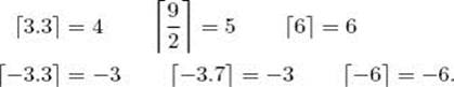
We call x the ceiling for x. For any integer n, n = n. We also sometimes need to refer to the largest integer that is less than or equal to a real number x. We denote that integer by x. For example,

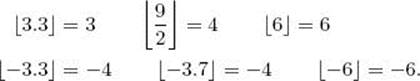
We call x the floor for x. For any integer n, n = n.

When we are able to determine only the approximate value of a desired result, we use the symbol ≈, which means “equals approximately.” For example, you should be familiar with the number π, which is used in the computation of the area and circumference of a circle. The value of π is not given by any finite number of decimal digits because we could go on generating more digits forever. (Indeed, there is not even a pattern as there is in Because the first six digits of π are 3.14159, we write

We use the symbol ≠ to mean “does not equal.” For example, if we want to state that the values of the variables x and y are not equal, we write

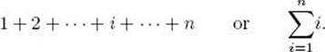
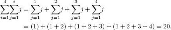
Often we need to refer to the sum of like terms. This is straightforward if there are not many terms. For example, if we need to refer to the sum of the first seven positive integers, we simply write

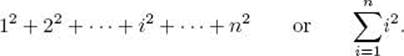
If we need to refer to the sum of the squares of the first seven positive integers, we simply write

This method works well when there are not many terms. However, it is not satisfactory if, for example, we need to refer to the sum of the first 100 positive integers. One way to do this is to write the first few terms, a general term, and the last term. That is, we write

If we need to refer to the sum of the squares of the first 100 positive integers, we could write

Sometimes when the general term is clear from the first few terms, we do not bother to write that term. For example, for the sum of the first 100 positive integers we could simply write

When it is instructive to show some of the terms, we write out some of them. However, a more concise method is to use the Greek letter Σ, which is pronounced sigma. For example, we use Σ to represent the sum of the first 100 positive integers as follows:

This notation means that while the variable i is taking values from 1 to 100, we are summing its values. Similarly, the sum of the squares of the first 100 positive integers can be represented by

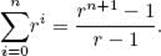
Often we want to denote the case in which the last integer in the sum is an arbitrary integer n. Using the methods just illustrated, we can represent the sum of the first n positive integers by

Similarly, the sum of the squares of the first n positive integers can be represented by

Sometimes we need to take the sum of a sum. For example,

Similarly, we can take the sum of a sum of a sum, and so on.

Finally, we sometimes need to refer to an entity that is larger than any real number. We call that entity infinity and denote it by ∞. For any real number x, we have

A.2 Functions

Very simply, a function f of one variable is a rule or law that associates with a value x a unique value f(x). For example, the function f that associates the square of a real number with a given real number x is

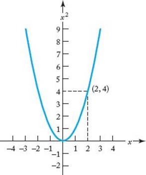
A function determines a set of ordered pairs. For example, the function f(x) = x² determines all the ordered pairs (x_, x²). A graph of a function is the set of all ordered pairs determined by the function. The graph of the function f(x) = x² appears in Figure A.1.

The function

is defined only if x ≠ 0. The domain of a function is the set of values for which the function is defined. For example, the domain of f(x) = 1/x is all real numbers other than 0, whereas the domain of f(x) = x² is all real numbers.

Figure A.1 The graph of the function f(x) = x². The ordered pair (2, 4) is illustrated.

Notice that the function

can assume only nonnegative values. By “nonnegative values” we mean values greater than or equal to 0, whereas by “positive values” we mean values strictly greater than 0. The range of a function is the set of values that the function can assume. The range of f(x) = x² is the nonnegative reals, the range of f(x) = 1/x is all real numbers other than 0, and the range of f(x) = (1/x)² is all positive reals. We say that a function is from its domain and to its range. For example, the function f(x) = x² is from the reals to the nonnegative reals.

A.3 Mathematical Induction

Some sums equal closed-form expressions. For example,

We can illustrate this equality by checking it for a few values of n, as follows:

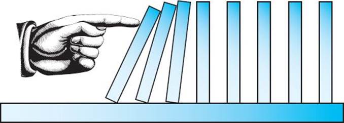
Figure A.2 If the first domino is knocked over, all the dominoes will fall.

However, because there are an infinite number of positive integers, we can never become certain that the equality holds for all positive integers n simply by checking individual cases. Checking individual cases can inform us only that the equality appears to be true. A powerful tool for obtaining a result for all positive integers n is mathematical induction.

Mathematical induction works in the same way as the domino principle. Figure A.2 illustrates that, if the distance between two dominoes is always less than the height of the dominoes, we can knock down all the dominoes merely by knocking over the first domino. We are able to do this because:

1. We knock over the first domino.

2. By spacing the dominoes so that the distance between any two of them is always less than their height, we guarantee that if the nth domino falls, the (n + 1)st domino will fall.

If we knock over the first domino, it will knock over the second, the second will knock over the third, and so on. In theory, we can have an arbitrarily large number of dominoes, and they all will fall.

An induction proof works in the same way. We first show that what we are trying to prove is true for n = 1. Next we show that if it is true for an arbitrary positive integer n, it must also be true for n + 1. Once we have shown this, we know that because it is true for n = 1, it must be true for n = 2; because it is true for n = 2, it must be true for n = 3; and so on, ad infinitum (to infinity). We can therefore conclude that it is true for all positive integers n. When using induction to prove that some statement concerning the positive integers is true, we use the following terminology:

The induction base is the proof that the statement is true for n = 1 (or some other initial value).

The induction hypothesis is the assumption that the statement is true for an arbitrary n ≥ 1 (or some other initial value).

The induction step is the proof that if the statement is true for n, it must also be true for n + 1.

The induction base amounts to knocking over the first domino, whereas the induction step shows that if the nth domino falls, the (n + 1)st domino will fall.

Example A.1

We show, for all positive integers n, that

Induction base: For n = 1,

Induction hypothesis: Assume, for an arbitrary positive integer n, that

Induction step: We need to show that

To that end,

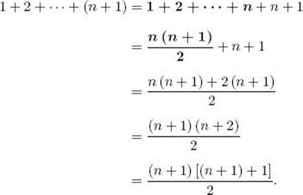
In the induction step, we highlight the terms that are equal by the induction hypothesis. We often do this to show where the induction hypothesis is being applied. Notice what is accomplished in the induction step. By assuming the induction hypothesis that

and doing some algebraic manipulations, we arrive at the conclusion that

Therefore, if the hypothesis is true for n, it must be true for n + 1. Because in the induction base we show that it is true for n = 1, we can conclude, using the domino principle, that it is true for all positive integers n.

You may wonder why we thought that the equality in Example A.1 might be true in the first place. This is an important point. We can often derive a possibly true statement by investigating some cases and making an educated guess. This is how the equality in Example A.1 was originally conceived. Induction can then be used to verify that the statement is true. If it is not true, of course, the induction proof fails. It is important to realize that it is never possible to derive a true statement using induction. Induction comes into play only after we have already derived a possibly true statement. In Section 8.5.4, we discuss constructive induction, which is a technique that can help us discover a true statement.

Another important point is that the initial value need not be n = 1. That is, the statement may be true only if n ≥ 10. In this case the induction base would be n = 10. In some cases our induction base is n = 0. This means we are proving the statement to be true for all nonnegative integers.

More examples of induction proofs follow.

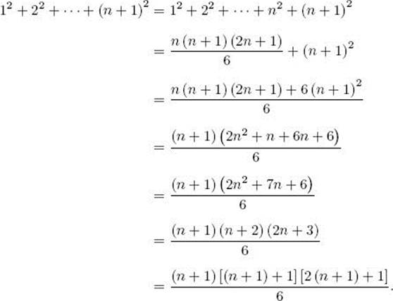
Example A.2

We show, for all positive integers n, that

Induction base: For n = 1,

Induction hypothesis: Assume, for an arbitrary positive integer n, that

Induction step: We need to show that

To that end,

In the next example, the induction base is n = 0.

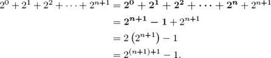
Example A.3

We show, for all nonnegative integers n, that

In summation notation, this equality is

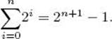
Induction base: For n = 0,

Induction hypothesis: Assume, for an arbitrary nonnegative integer n, that

Induction step: We need to show that

To that end,

Example A.3 is a special case of the result in the next example.

Example A.4

We show, for all nonnegative integers n and real numbers r ≠ 1, that

The terms in this sum are called a geometric progression.

Induction base: For n = 0,

Induction hypothesis: Assume, for an arbitrary nonnegative integer n, that

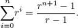
Induction step: We need to show that

To that end,

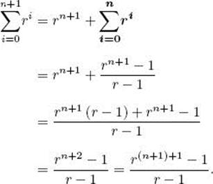
Sometimes results that can be obtained using induction can be established more readily in another way. For instance, the preceding example showed that

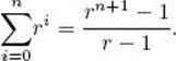
Instead of using induction, we can multiply the expression on the left in the preceding equality by the denominator on the right and simplify, as follows:

Dividing both sides of this equality by r − 1 gives the desired result.

We present one more example of induction.

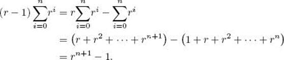
Example A.5

We show, for all positive integers n, that

Induction base: For n = 1,

Induction hypothesis: Assume, for an arbitrary positive integer n, that

Induction step: We need to show that

To that end,

Another way to make the induction hypothesis is to assume that the statement is true for all k greater than or equal to the initial value and less than n, and then, in the induction step, prove that it is true for n. We do this in the proof of Theorem 1.1 in Section 1.2.2.

Although our examples have all involved the determination of closed-form expressions for sums, there are many other induction applications. We encounter some of them in this text.

A.4 Theorems and Lemmas

The dictionary defines a theorem as a proposition that sets forth something to be proved. It has the same meaning in mathematics. Each of the examples in the preceding section could be stated as a theorem, whereas the induction proof constitutes a proof of the theorem. For example, we could state Example A.1 as follows:

Theorem A.1

For all integers n > 0, we have

Proof: The proof would go here. In this case, it would be the induction proof used in Example A.1.

Usually the purpose of stating and proving a theorem is to obtain a general result that can be applied to many specific cases. For example, we can use Theorem A.1 to quickly calculate the sum of the first n integers for any positive integer n.

Sometimes students have difficulty understanding the difference between a theorem that is an “if” statement and one that is an “if and only if” statement. The following two theorems illustrate this difference.

Theorem A.2

For any real number x, if x > 0, then x² > 0.

Proof: The theorem follows from the fact that the product of two positive numbers is positive.

The reverse of the implication stated in Theorem A.2 is not true. That is, it is not true that if x² > 0, then x > 0. For example,

and −3 is not greater than 0. Indeed, the square of any negative number is greater than 0. Therefore, Theorem A.2 is an example of an “if ” statement.

When the reverse implication is also true, the theorem is an “if and only if ” statement, and it is necessary to prove both the implication and the reverse implication. The following theorem is an example of an “if and only if ” statement.

Theorem A.3

For any real number x, x > 0 if and only if 1/x > 0.

Proof: Prove the implication. Suppose that x > 0. Then

because the quotient of two positive numbers is greater than 0.

Prove the reverse implication. Suppose that 1/x > 0. Then

again because the quotient of two positive numbers is greater than 0.

The dictionary defines a lemma as a subsidiary proposition employed to prove another proposition. Like a theorem, a lemma is a proposition that sets forth something to be proved. However, we usually do not care about the proposition in the lemma for its own sake. Rather, when the proof of a theorem relies on the truth of one or more auxiliary propositions, we often state and prove lemmas concerning those propositions. We then employ those lemmas to prove the theorem.

A.5 Logarithms

Logarithms are one of the mathematical tools used most in analysis of algorithms. We briefly review their properties.

• A.5.1 Definition and Properties of Logarithms

The common logarithm of a number is the power to which 10 must be raised to produce the number. If x is a given number, we denote its common logarithm by log x.

Example A.6

Some common logarithms follow:

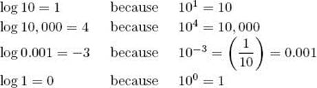
Recall that the value of any nonzero number raised to the 0th power is 1.

In general, the logarithm of a number x is the power to which another number a, called the base, must be raised to produce x. The number a can be any positive number other than 1, whereas x must be positive. That is, there is no such thing as the logarithm of a negative number or of 0. In symbols, we write log_a x.

Example A.7

Some examples of log_a x follow:

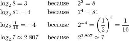
Notice that the last result in Example A.7 is for a number that is not an integral power of the base. Logarithms exist for all positive numbers, not just for integral powers of the base. A discussion of the meaning of the logarithm when the number is not an integral power of the base is beyond the scope of this appendix. We note here only that the logarithm is an increasing function. That is,

Therefore,

We saw in Example A.7 that log₂7 is about 2.807, which is between 2 and 3.

Listed below are some important properties of logarithms that are useful in the analysis of algorithms.

Some Properties of Logarithms (In all cases, a > 1, b > 1, x > 0, and y > 0):

1. log_a1 = 0

2. a^log_a^x = x

3. log_a (xy) = log_ax + log_a y

4.

5. log_a x^y = ylog_ax

6. x^log_a^y = y^log_a^x

7.

Example A.8

Some examples of applying the previous properties follow:

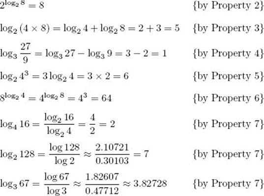
Because many calculators have a log function (recall that log means log₁₀), the last two results in Example A.8 show how one can use a calculator to compute a logarithm for an arbitrary base. (This is how we computed them.)

We encounter the logarithm to base 2 so often in analysis of algorithms that we give it its own simple symbol. That is, we denote log₂ x by lg x. From now on, we use this notation.

• A.5.2 The Natural Logarithm

You may recall the number e, whose value is approximately 2.718281828459. Like π, the number e cannot be expressed exactly by any finite number of decimal digits, and indeed there is not even a repeating pattern of digits in its decimal expansion. We denote log_e x by ln x, and we call it thenatural logarithm of x. For example,

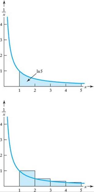
You may wonder where we got this answer. We simply used a calculator that has an ln function. Without studying calculus, it is not possible to understand how the natural logarithm is computed and why it is called “natural.” Indeed, when we merely look at e, the natural logarithm appears most unnatural. Although a discussion of calculus is beyond our present scope (except for some material marked), we do want to explore one property of the natural logarithm that is important to the analysis of algorithms. With calculus it is possible to show that ln x is the area under the curve 1/x that lies between 1 and x. This is illustrated in the top graph in Figure A.3 for x = 5. In the bottom graph in that figure, we show how that area can be approximated by summing the areas of rectangles that are each one unit wide. The graph shows that the approximation to ln 5 is

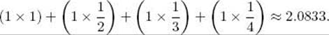
Notice that this area is always larger than the true area. Using a calculator, we can determine that

The area of the rectangles is not a very good approximation to ln 5. However, by the time we get to the last rectangle (the one between the x-values 4 and 5), the area is not much different from the area under the curve between x = 4 and x = 5. This is not the case for the first rectangle. Each successive rectangle gives a better approximation than its predecessor. Therefore, when the number is not small, the sum of the areas of the rectangles is close to the value of the natural logarithm. The following example shows the usefulness of this result.

Figure A.3 The shaded area in the top graph is ln 5. The combined area of the shaded rectangles in the bottom graph is an approximation to ln 5.

Example A.9

Suppose we wish to compute

There is no closed-form expression for this sum. However, in accordance with the preceding discussion, if n is not small,

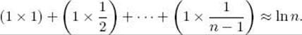
When n is not small, the value of 1/n is negligible in comparison with the sum. Therefore, we can also add that term to get the result

We will use this result in some of our analyses. In general, it is possible to show that

A.6 Sets

Informally, a set is a collection of objects. We denote sets by capital letters such as S, and, if we enumerate all the objects in a set, we enclose them in braces. For example,

is the set containing the first four positive integers. The order in which we list the objects is irrelevant. This means that

are the same set—namely, the set of the first four positive integers. Another example of a set is

This is the set of the names of the days in the week. When a set is infinite, we can represent the set using a description of the objects in the set. For example, if we want to represent the set of positive integers that are integral multiples of 3, we can write

Alternatively, we can show some items and a general item, as follows:

The objects in a set are called elements or members of the set. If x is an element of the set S, we write x S. If x is not an element of S, we write x S. For example,

We say that the sets S and T are equal if they have the same elements, and we write S = T. If they are not equal, we write S ≠ T. For example,

If S and T are two sets such that every element in S is also in T, we say that S is a subset of T, and we write S T. For example,

Every set is a subset of itself. That is, for any set S, S ⊆ S. If S is a subset of T that is not equal to T, we say that S is a proper subset of T, and we write S ⊂ T. For example,

For two sets S and T, the intersection of S and T is defined as the set of all elements that are in both S and T. We write S ∩ T. For example,

For two sets S and T, the union of S and T is defined as the set of all elements that are in either S or T. We write S T. For example,

For two sets S and T, the difference between S and T is defined as the set of all elements that are in S but not in T. We write S − T. For example,

The empty set is defined as the set containing no elements. We denote the empty set by Ø.

The universal set U is defined as the set consisting of all elements under consideration. This means that if S is any set we are considering, then S ⊆ U. For example, if we are considering sets of positive integers, then

A.7 Permutations and Combinations

Suppose we have four balls marked A, B, C, and D in an urn or container, and two balls will be drawn from the urn. To win a lottery, we must pick the balls in the order in which they are drawn. To gain insight into the likelihood of our winning, we should determine how many outcomes are possible. The possible outcomes are:

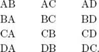
The outcomes AB and BA, for example, are different because we must pick the balls in the correct order. We have listed 12 different outcomes. However, can we be sure that these are all the outcomes? Notice that we arranged the outcomes in four rows and three columns. Each row corresponds to a distinct choice for the first ball; there are four such choices. Once we have made that choice, the second letters in the entries in a row correspond to the remaining distinct choices for the second ball; there are three such choices. The total number of outcomes is therefore

This result can be generalized. For example, if we have four balls and three are drawn, the first ball can be any one of four; once the first ball is drawn, the second ball can be any of three; and once the second ball is drawn, the third ball can be any of two. The number of outcomes is therefore

In general, if we have n balls, and we are picking k of them, the number of possible outcomes is

This is called the number of permutations of n objects taken k at a time. If n = 4 and k = 3, this formula yields

which is the result already obtained. If n = 10 and k = 5, the formula yields

If k = n, we are picking all the balls. This is simply called the number of permutations of n objects. The previous formula shows that it is given by

Recall that for a positive integer n, n! is defined as the integer times all the positive integers less than it, the value of 0! is defined to be 1, and n! is not defined for negative integers.

Next consider a lottery that we can win by merely picking the correct balls. That is, we do not have to get the order right. Suppose again that there are four balls marked A, B, C, and D, and two are drawn. Each outcome in this lottery corresponds to two outcomes in the previous lottery. For example, the outcomes AB and BA in the other lottery are both the same for the purposes of this lottery. We will call this outcome

Because two outcomes in the previous lottery correspond to one outcome in this lottery, we can determine how many outcomes there are in this lottery by dividing the number of outcomes in the previous lottery by 2. This means that there are

outcomes in this lottery. The six distinct outcomes are

Suppose now that three balls are drawn from the urn containing the four balls marked A, B, C, and D, and we do not have to get the order right. Then the following outcomes are all the same for the purposes of this lottery:

These outcomes are simply the permutations of three objects. Recall that the number of such permutations is given by 3! = 6. To determine how many distinct outcomes there are in this lottery, we need to divide by 3! the number of distinct outcomes in the lottery, where the order does matter. That is, there are

outcomes in this lottery. They are

In general, if there are n balls and k balls are drawn and the order does not matter, the number of distinct outcomes is given by

This is called the number of combinations of n objects taken k at a time. Because

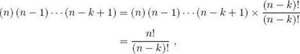
the formula for the number of combinations of n objects taken k at a time is usually shown as

Using this formula, the number of combinations of eight objects taken three at a time is given by

The Binomial theorem, which is proven in algebra texts, states that for any nonnegative integer n and real numbers a and b,

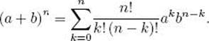
Because the number of combinations of n objects taken k at a time is the coefficient of a^kb^n−k in this expression, that number is called the binomial coefficient. We will denote it

Example A.10

We show that the number of subsets, including the empty set, of a set containing n items is 2ⁿ. For 0 ≤ k ≤ n, the number of subsets of size k is the number of combinations of n objects taken k at a time, which is .This means that the total number of subsets is

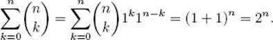
The second-to-last equality is by the Binomial theorem.

A.8 Probability

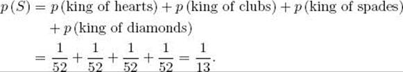
You may recall using probability theory in situations such as drawing a ball from an urn, drawing the top card from a deck of playing cards, and tossing a coin. We call the act of drawing a ball, drawing the top card, or tossing a coin an experiment. In general, probability theory is applicable when we have an experiment that has a set of distinct outcomes that we can describe. The set of all possible outcomes is called a sample space or population. Mathematicians usually say “sample space,” whereas social scientists usually say “population” (because they study people). We use these terms interchangeably. Any subset of a sample space is called an event. A subset containing only one element is called an elementary event.

Example A.11

In the experiment of drawing the top card from an ordinary deck of playing cards, the sample space contains the 52 different cards. The set

is an event, and the set

is an elementary event. There are 52 elementary events in the sample space.

The meaning of an event (subset) is that one of the elements in the subset is the outcome of the experiment. In Example A.11, the meaning of the event S is that the card drawn is any one of the four kings, and the meaning of the elementary event E is that the card drawn is the king of hearts.

We measure our certainty that an event contains the outcome of the experiment with a real number called the probability of the event. The following is a general definition of probability when the sample space is finite.

Definition

Suppose we have a sample space containing n distinct outcomes:

A function that assigns a real number p (S) to each event S is called a probability function if it satisfies the following conditions:

1. 0 ≤ p (e_i) ≤ 1 for 1 ≤ i ≤ n

2. p (e₁) + p (e₂) + · · · + p (e_n) = 1

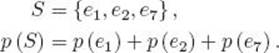
3. For each event S that is not an elementary event, p (S) is the sum of the probabilities of the elementary events whose outcomes are in S. For example, if

The sample space along with the function p is called a probability space.

Because we define probability as a function of a set, we should write p ({e_i}) instead of p (e_i) when referring to the probability of an elementary event. However, to avoid clutter, we do not do this. In the same way, we do not use the braces when referring to the probability of an event that is not elementary. For example, we write p (e₁, e₂, e₇) for the probability of the event {e₁, e₂, e₇}.

We can associate an outcome with the elementary event containing that outcome, and therefore we can speak of the probability of an outcome. Clearly, this means the probability of the elementary event containing the outcome.

The simplest way to assign probabilities is to use the Principle of Indifference. This principle says that outcomes are to be considered equiprobable if we have no reason to expect or prefer one over the other. According to this principle, when there are n distinct outcomes, the probability of each of them is the ratio 1/n.

Example A.12

Suppose we have four balls marked A, B, C, and D in an urn, and the experiment is to draw one ball. The sample space is {A, B, C, D}, and, according to the Principle of Indifference,

The event {A, B} means that either ball A or ball B is drawn. Its probability is given by

Example A.13

Suppose we have the experiment of drawing the top card from an ordinary deck of playing cards. Because there are 52 cards, according to the Principle of Indifference, the probability of each card is . For example,

The event

means that the card drawn is a king. Its probability is given by

Sometimes we can compute probabilities using the formulas for permutations and combinations given in the preceding section. The following example shows how this is done.

Example A.14

Suppose there are five balls marked A, B, C, D, and E in an urn, and the experiment is to draw three balls and the order does not matter. We will compute p(A and B and C). Recall that by “A and B and C” we mean the outcome that A, B, and C are picked in any order. To determine the probability using the Principle of Indifference, we need to compute the number of distinct outcomes. That is, we need the number of combinations of five objects taken three at a time. Using the formula in the preceding section, that number is given by

Therefore, according to the Principle of Indifference,

which is the same as the probabilities of the other nine outcomes.

Too often, students, who do not have the opportunity to study probability theory in depth, are left with the impression that probability is simply about ratios. It would be unfair, even in this cursory overview, to give this impression. In fact, most important applications of probability have nothing to do with ratios. To illustrate, we give two simple examples.

A classic textbook example of probability involves tossing a coin. Because of the symmetry of a coin, we ordinarily use the Principle of Indifference to assign probabilities. Therefore, we assign

On the other hand, we could toss a thumbtack. Like a coin, a thumbtack can land in two ways. It can land on its flat end (head) or it can land with the edge of the flat end (and the point) touching the ground. We assume that it cannot land only on its point. These two ways of landing are illustrated in Figure A.4. Using coin terminology, we will call the flat end “heads” and the other outcome “tails.” Because the thumbtack lacks symmetry, there is no reason to use the Principle of Indifference and assign the same probability to heads and tails. How then do we assign probabilities? In the case of a coin, when we say , we are implicitly assuming that if we tossed the coin 1,000 times, it should land on its head about 500 times. Indeed, if it only landed on its head 100 times, we would become suspicious that it was unevenly weighted and that the probability was not . This notion of repeatedly performing the same experiment gives us a way of actually computing a probability. That is, if we repeat an experiment many times, we can be fairly certain that the probability of an outcome is about equal to the fraction of times the outcome actually occurs. (Some philosophers actually define probability as the limit of this fraction as the number of trials approaches infinity.) For example, one of our students tossed a thumbtack 10,000 times and it landed on its flat end (heads) 3,761 times. Therefore, for that tack,

Figure A.4 The two ways a thumbtack can land. Because of the asymmetry of a thumbtack, these two ways do not necessarily have the same probability.

We see that the probabilities of the two events need not be the same, but that the probabilities still sum to 1. This way of determining probabilities is called the relative frequency approach to probability. When probabilities are computed from the relative frequency, we use the ≈ symbol because we cannot be certain that the relative frequency is exactly equal to the probability regardless of how many trials are performed. For example, suppose we have two balls marked A and B in an urn and we repeat the experiment of picking one ball 10,000 times. We cannot be certain that the ball marked A will be picked exactly 5,000 times. It may be picked only 4,967 times. Using the Principle of Indifference, we would have

whereas using the relative frequency approach we would have

The relative frequency approach is not limited to experiments with only two possible outcomes. For example, if we had a six-sided die that was not a perfect cube, the probabilities of the six elementary events could all be different. However, they would still sum to 1. The following example illustrates this situation.

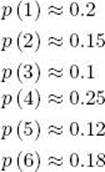
Example A.15

Suppose we have an asymmetrical six-sided die, and in 1,000 throws we determine that the six sides come up the following numbers of times:

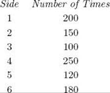
Then

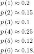
By Condition 3 in the definition of a probability space,

This is the probability that either a 2 or a 3 comes up in a throw of the die.

There are other approaches to probability, not the least of which is the notion of probability as a degree of belief in an outcome. For example, suppose the Chicago Bears were going to play the Dallas Cowboys in a football game. At the time this text is being written, one of its authors has little reason to believe that the Bears would win. Therefore, he would not assign equal probabilities to each team winning. Because the game could not be repeated many times, he could not obtain the probabilities using the relative frequency approach. However, if he was going to bet on the game, he would want to access the probability of the Bears winning. He could do so using the subjectivistic approach to probability. One way to access probabilities using this approach is as follows: If a lottery ticket for the Bears winning cost $1, an individual would determine how much he or she felt the ticket should be worth if the Bears did win. One of the authors feels that it would have to be worth $5. This means that he would be willing to pay $1 for the ticket only if it would be worth at least $5 in the event that the Bears won. For him, the probability of the Bears winning is given by

That is, the probability is computed from what he believes would be a fair bet. This approach is called “subjective” because someone else might say that the ticket would need to be worth only $4. For that person, p(Bears win) = 0.25. Neither person would be logically incorrect. When a probability simply represents an individual’s belief, there is no unique correct probability. A probability is a function of the individual’s beliefs, which means it is subjective. If someone believed that the amount won should be the same as the amount bet (that is, that the ticket should be worth $2), then for that person

We see that probability is much more than ratios. You should read Fine (1973) for a thorough coverage of the meaning and philosophy of probability. The relative frequency approach to probability is discussed in Neapolitan (1992). The expression “Principle of Indifference” first appeared in Keynes (1948) (originally published in 1921). Neapolitan (1990) discusses paradoxes resulting from use of the Principle of Indifference.

• A.8.1 Randomness

Although the term “random” is used freely in conversation, it is quite difficult to define rigorously. Randomness involves a process. Intuitively, by a random process we mean the following. First, the process must be capable of generating an arbitrarily long sequence of outcomes. For example, the process of repeatedly tossing the same coin can generate an arbitrarily long sequence of outcomes that are either heads or tails. Second, the outcomes must be unpredictable. What it means to be “unpredictable,” however, is somewhat vague. It seems we are back where we started; we have simply replaced “random” with “unpredictable.”

In the early part of the 20th century, Richard von Mises made the concept of randomness more concrete. He said that an “unpredictable” process should not allow a successful gambling strategy. That is, if we chose to bet on an outcome of such a process, we could not improve our chances of winning by betting on some subsequence of the outcomes instead of betting on every outcome. For example, suppose we decided to bet on heads in the repeated tossing of a coin. Most of us feel that we could not improve our chances by betting on every other toss instead of on every toss. Furthermore, most of us feel that there is no other “special” subsequence that could improve our chances. If indeed we could not improve our chances by betting on some subsequence, then the repeated tossing of the coin would be a random process. As another example, suppose that we repeatedly sampled individuals from a population that contained individuals with and without cancer and that we put each sampled individual back into the population before sampling the next individual. (This is called sampling with replacement.) Let’s say we chose to bet on cancer. If we sampled in such a way as to never give preference to any particular individual, most of us feel that we would not improve our chances by betting only on some subsequence instead of betting every time. If indeed we could not improve our chances by betting on some subsequence, then the process of sampling would be random. However, if we sometimes gave preference to individuals who smoked by sampling every fourth time only from smokers, and we sampled the other times from the entire population, the process would no longer be random because we could improve our chances by betting every fourth time instead of every time.

Intuitively, when we say that “we sample in such a way as to never give preference to any particular individual,” we mean that there is no pattern in the way the sampling is done. For example, if we were sampling balls with replacement from an urn, we would never give any ball preference if we shook the urn vigorously to thoroughly mix the balls before each sample. You may have noticed how thoroughly the balls are mixed before they are drawn in state lotteries. When sampling is done from a human population, it is not as easy to ensure that preference is not given. The discussion of sampling methods is beyond the scope of this appendix.

Von Mises’ requirement of not allowing a successful gambling strategy gives us a better grasp of the meaning of randomness. A predictable or nonrandom process does allow a successful gambling strategy. One example of a nonrandom process is the one mentioned above in which we sampled every fourth time from smokers. A less obvious example concerns the exercise pattern of one of the authors. He prefers to exercise at his health club on Tuesday, Thursday, and Sunday, but if he misses a day he makes up for it on one of the other days. If we were going to bet on whether he exercises on a given day, we could do much better by betting every Tuesday, Thursday, and Sunday than by betting every day. This process is not random.

Even though Von Mises was able to give us a better understanding of randomness, he was not able to create a rigorous, mathematical definition. Andrei Kolmogorov eventually did so with the concept of compressible sequences. Briefly, a finite sequence is defined as compressible if it can be encoded in fewer bits than it takes to encode every item in the sequence. For example, the sequence

which is simply “1 0” repeated 16 times, can be represented by

Because it takes fewer bits to encode this representation than it does to encode every item in the sequence, the sequence is compressible. A finite sequence that is not compressible is called a random sequence. For example, the sequence

is random because it does not have a more efficient representation. Intuitively, a random sequence is one that shows no regularity or pattern.

According to the Kolmogorov theory, a random process is a process that generates a random sequence when the process is continued long enough. For example, suppose we repeatedly toss a coin, and associate 1 with heads and 0 with tails. After six tosses we may see the sequence

but, according to the Kolmogorov theory, eventually the entire sequence will show no such regularity. There is some philosophical difficulty with defining a random process as one that definitely generates a random sequence. Many probabilists feel that it is only highly probable that the sequence will be random, and that the possibility exists that the sequence will not be random. For example, in the repeated tossing of a coin, they believe that, although it is very unlikely, the coin could come up heads forever. As mentioned previously, randomness is a difficult concept. Even today there is controversy over its properties.

Let’s discuss how randomness relates to probability. A random process determines a probability space (see definition given at the beginning of this section), and the experiment in the space is performed each time the process generates an outcome. This is illustrated by the following examples.

Example A.16

Suppose we have an urn containing one black ball and one white ball, and we repeatedly draw a ball and replace it. This random process determines a probability space in which

We perform the experiment in the space each time we draw a ball.

Example A.17

The repeated throwing of the asymmetrical six-sided die in Example A.15 is a random process that determines a probability space in which

We perform the experiment in the space each time we throw the die.

Example A.18

Suppose we have a population of n people, some of whom have cancer, we sample people with replacement, and we sample in such a way as to never give preference to any particular individual. This random process determines a probability space in which the population is the sample space (recall that “sample space” and “population” can be used interchangeably) and the probability of each person being sampled (elementary event) is 1/n. The probability of a person with cancer being sampled is

Each time we perform the experiment, we say that we sample (pick) a person at random from the population. The set of outcomes in all repetitions of the experiment is called a random sample of the population. Using statistical techniques, it can be shown that if a random sample is large, then it is highly probable that the sample is representative of the population. For example, if the random sample is large, and of the people sampled have cancer, it is highly probable that the fraction of people in the population with cancer is close to .

Example A.19

Suppose we have an ordinary deck of playing cards, and we turn over the cards in sequence. This process is not random, and the cards are not picked at random. This nonrandom process determines a different probability space each time an outcome is generated. On the first trial, each card has a probability of . On the second trial, the card turned over in the first trial has a probability of 0 and each of the other cards has a probability of , and so on.

Suppose we repeatedly draw the top card, replace it, and shuffle once. Is this a random process and are the cards picked at random? The answer is no. The magician and statistician Persi Diaconis has shown that the cards must be shuffled seven times to thoroughly mix them and make the process random (see Aldous and Diaconis, 1986).

Although von Mises’ notion of randomness is intuitively very appealing today, his views were not widely held at the time he developed his theory (in the early part of the 20th century). His strongest opponent was the philosopher K. Marbe. Marbe held that nature is endowed with a memory. According to his theory, if tails comes up 15 consecutive times in repeated tosses of a fair coin—that is, a coin for which the relative frequency of heads is 0.5—the probability of heads coming up on the next toss is increased because nature will compensate for all the previous tails. If this theory were correct, we could improve our chances of winning by betting on heads only after a long sequence of tails. Iverson et al. (1971) conducted experiments that substantiated the views of von Mises and Kolmogorov. Specifically, their experiments showed that coin tosses and dice throws do generate random sequences. Today few scientists subscribe to Marbe’s theory, although quite a few gamblers seem to.

Von Mises’ original theory appeared in von Mises (1919) and is discussed more accessibly in von Mises (1957). A detailed coverage of compressible sequences and random sequences can be found in Van Lambalgen (1987). Neapolitan (1992) and Van Lambalgen (1987) both address the difficulties in defining a random process as one that definitely generates a random sequence.

• A.8.2 The Expected Value

We introduce the expected value (average) with an example.

Example A.20

Suppose we have four students with heights of 68, 72, 67, and 74 inches. Their average height is given by

Suppose now that we have 1,000 students whose heights are distributed according to the following percentages:

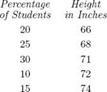
To compute the average height, we could first determine the height of each student and proceed as before. However, it is much more efficient to simply obtain the average as follows:

Notice that the percentages in this example are simply probabilities obtained using the Principle of Indifference. That is, the fact that 20% of the students are 66 inches tall means that 200 students are 66 inches tall, and if we pick a student at random from the 1,000 students, then

In general, the expected value is defined as follows.

Definition

Suppose we have a probability space with the sample space

and each outcome e_i has a real number f(e_i) associated with it. Then f(e_i) is called a random variable on the sample space, and the expected value, or average, of f(e_i) is given by

Random variables are called “random” because random processes can determine the values of random variables. The terms “chance variable” and “stochastic variable” are also used. We use “random variable” because it is the most popular.

Example A.21

Suppose we have the asymmetrical six-sided die in Example A.15. That is,

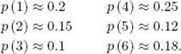
Our sample space consists of the six different sides that can come up, a random variable on this sample space is the number written on the side, and the expected value of this random variable is

If we threw the die many times, we would expect the average of the numbers showing up to equal about 3.48.

A sample space does not have a unique random variable defined on it. Another random variable on this sample space might be the function that assigns 0 if an odd number comes up and 1 if an even number comes up. The expected value of this random variable is

Example A.22

Suppose the 1,000 students in Example A.20 are our sample space. The height, as computed in Example A.20, is one random variable on this sample space. Another one is the weight. If the weights are distributed according to the following percentages:

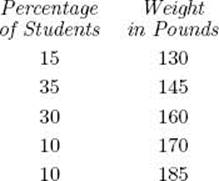
the expected value of this random variable is

EXERCISES

Section A.1

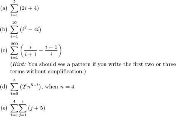
1. Determine each of the following

(a) [2.8]

(b) [−10.42]

(c) [4.2]

(d) [−34.92]

(f) [2π]

2. Show that [n] = − [−n].

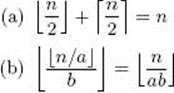
3. Show that, for any real x,

4. Show that for any integers a > 0, b > 0, and n,

5. Write each of the following using summation (sigma) notation.

(a) 2 + 4 + 6 + · · · + 2 (99) + 2 (100)

(b) 2 + 4 + 6 + · · · + 2 (n − 1) + 2n

(c) 3 + 12 + 27 + · · · + 1200

6. Evaluate each of the following sums.

Section A.2

7. Graph the function What are the domain and range of this function?

8. Graph the function f(x) = (x – 2) / (x + 5). What are the domain and range of this function?

9. Graph the function f(x) = x. What are the domain and range of this function?

10. Graph the function f(x) = x. What are the domain and range of this function?

Section A.3

11. Use mathematical induction to show that, for all integers n > 0,

12. Use mathematical induction to show that n² − n is even for any positive integer n.

13. Use mathematical induction to show that, for all integers n > 4,

14. Use mathematical induction to show that, for all integers n > 0,

Section A.4

15. Prove that if a and b are both odd integers, a + b is an even integer. Is the reverse implication true?

16. Prove that a + b is an odd integer if and only if a and b are not both odd or both even integers.

Section A.5

17. Determine each of the following.

(a) log 1, 000 (b) log 100, 000

(c) log₄ 64

(d)

(e) log₅ 125

(f) log 23

(g) lg (16 × 8)

(h) log (1,000/100, 000)

(i) 2^{lg 125}

18. Graph f(x) = 2^x and g (x) = lg x on the same coordinate system.

19. Give the values of x for which x² + 6x + 12 > 8x + 20.

20. Give the values of x for which x > 500 lg x.

21. Show that f(x) = 2^{3 lg x} is not an exponential function.

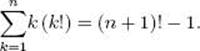
22. Show that, for any positive integer n,

23. Find a formula for lg (n!) using Stirling’s approximation for n!,

for large n.

Section A.6

24. Let U = {2, 4, 5, 6, 8, 10, 12}, S = {2, 4, 5, 10}, and T = {2, 6, 8, 10}. (U is the universal set.) Determine each of the following.

(a) S T

(b) S ∩ T

(c) S – T

(d) T – S

(e) ((S ∩ T) S)

(f) U − S (called the complement of S)

25. Given that the set S contains n elements, show that S has 2ⁿ subsets.

26. Let |S| stand for the number of elements in S. Show the validity of

27. Show that the following are equivalent.

(a) S ⊂ T

(b) S ∩ T = S

(c) S T = T

Section A. 7

28. Determine the number of permutations of 10 objects taken six at a time.

29. Determine the number of combinations of 10 objects taken six at a time. That is, determine

30. Suppose there is a lottery in which four balls are drawn from an urn containing 10 balls. A winning ticket must show the balls in the order in which they are drawn. How many distinguishable tickets exist?

31. Suppose there is a lottery in which four balls are drawn from a bin containing 10 balls. A winning ticket must merely show the correct balls without regard for the order in which they are drawn. How many distinguishable tickets exist?

32. Use mathematical induction to prove the Binomial theorem, given in Section A.7.

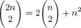
33. Show the validity of the following identity.

34. Assume that we have k₁ objects of the first kind, k₂ objects of the second kind,…, and k_m objects of the mth kind, where k₁ + k₂ + · · · + k_m = n. Show that the number of distinguishable permutations of these n objects is equal to

35. Let f(n, m) be the number of ways to distribute n identical objects into m sets, where the ordering of the sets matters. For example, if n = 4, m = 2, and our set of objects is {A, A, A, A}, the possible distributions are as follows:

1. {A, A, A, A}, Ø

2. {A, A, A}, {A}

3. {A, A}, {A, A}

4. {A}, {A, A, A}

5. Ø, {A, A, A, A}

We see that f(4, 2) = 5. Show that in general

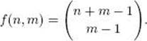
Hint: Not that the set of all such distributions consists of all those that have n A’s in the first slot, all those that have n − 1 A’s in the first slot,..., and all those that have 0 A’s in the first slot. The use induction on m.

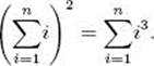
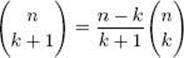
36. Show the validity of the following identity.

Section A.8

37. Suppose we have the lottery in Exercise 30. Assume all possible tickets are printed and all tickets are distinct.

(a) Compute the probability of winning if one ticket is purchased.

(b) Compute the probability of winning if seven tickets are purchased.

38. Suppose a poker hand (five cards) is dealt from an ordinary deck (52 cards).

(a) Compute the probability of the hand containing four aces.

(b) Compute the probability of the hand containing four of a kind.

39. Suppose a fair six-sided die (that is, the probability of each side turning up is ) is to be rolled. The player will receive an amount of dollars equal to the number of dots that turn up, except when five or six dots turn up, in which case the player will lose $5 or $6, respectively.

(a) Compute the expected value of the amount of money the player will win or lose.

(b) If the game is repeated 100 times, compute the most money the player will lose, the most money the player will win, and the amount the player can expect to win or lose.

40. Assume we are searching for an element in a list of n distinct elements. What is the average (expected) number of comparisons required when the Sequential Search algorithm (linear search) is used?

41. What is the expected number of movements of elements in a delete operation on an array of n elements?