Foundations of Algorithms (2015)

Chapter 5 Backtracking

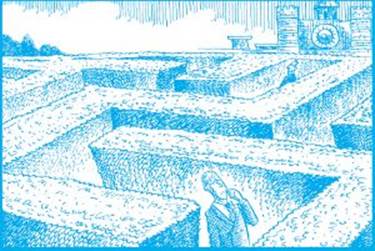
If you were trying to find your way through the well-known maze of hedges by Hampton Court Palace in England, you would have no choice but to follow a hopeless path until you reached a dead end. When that happened, you’d go back to a fork and pursue another path. Anyone who has ever tried solving a maze puzzle has experienced the frustration of hitting dead ends. Think how much easier it would be if there were a sign, positioned a short way down a path, that told you that the path led to nothing but dead ends. If the sign were positioned near the beginning of the path, the time savings could be enormous, because all forks after that sign would be eliminated from consideration. This means that not one but many dead ends would be avoided. There are no such signs in the famous maze of hedges or in most maze puzzles. However, as we shall see, they do exist in backtracking algorithms.

Backtracking is very useful for problems such a the 0-1 Knapsack problem. Although in Section 4.5.3 we found a dynamic programming algorithm for this problem that is efficient if the capacity W of the knapsack is not large, the algorithm is still exponential-time in the worst case. The 0-1 Knapsack problem is in the class of problems discussed in Chapter 9. No one has ever found algorithms for any of those problems whose worst-case time complexities are better than exponential, but no one has ever proved that such algorithms are not possible. One way to try to handle the 0-1 Knapsack problem would be to actually generate all the subsets, but this would be like following every path in a maze until a dead end is reached. Recall from Section 4.5.1 that there are 2ⁿ subsets, which means that this brute-force method is feasible only for small values of n. However, if while generating the subsets we can find signs that tell us that many of them need not be generated, we can often avoid much unnecessary labor. This is exactly what a backtracking algorithm does. Backtracking algorithms for problems such as the 0-1 Knapsack problem are still exponential-time (or even worse) in the worst case. They are useful because they are efficient for many large instances, not because they are efficient for all large instances. We return to the 0-1 Knapsack problem in Section 5.7. Before that, we introduce backtracking with a simple example in Section 5.1 and solve several other problems in the other sections.

5.1 The Backtracking Technique

Backtracking is used to solve problems in which a sequence of objects is chosen from a specified set so that the sequence satisfies some criterion. The classic example of the use of backtracking is in the n-Queens problem. The goal in this problem is to position n queens on an n×n chessboard so that no two queens threaten each other; that is, no two queens may be in the same row, column, or diagonal. The sequence in this problem is the n positions in which the queens are placed, the set for each choice is the n² possible positions on the chessboard, and the criterion is that no two queens can threaten each other. The n-Queens problem is a generalization of its instance when n = 8, which is the instance using a standard chessboard. For the sake of brevity, we will illustrate backtracking using the instance when n = 4.

Backtracking is a modified depth-first search of a tree (here “tree” means a rooted tree). So let’s review the depth-first search before proceeding. Although the depth-first search is defined for graphs in general, we will discuss only searching of trees, because backtracking involves only a tree search. A preorder tree traversal is a depth-first search of the tree. This means that the root is visited first, and a visit to a node is followed immediately by visits to all descendants of the node. Although a depth-first search does not require that the children be visited in any particular order, we will visit the children of a node from left to right in the applications in this chapter.

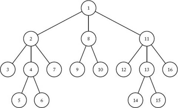
Figure 5.1 shows a depth-first search of a tree performed in this manner. The nodes are numbered in the order in which they are visited. Notice that in a depth-first search, a path is followed as deeply as possible until a dead end is reached. At a dead end we back up until we reach a node with an unvisited child, and then we again proceed to go as deep as possible.

Figure 5.1 A tree with nodes numbered according to a depth-first search.

There is a simple recursive algorithm for doing a depth-first search. Because we are presently interested only in preorder traversals of trees, we give a version that specifically accomplishes this. The procedure is called by passing the root at the top level.

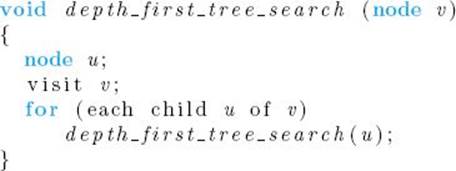
This general-purpose algorithm does not state that the children must be visited in any particular order. However, as mentioned previously, we visit them from left to right.

Now let’s illustrate the backtracking technique with the instance of the n-Queens problem when n = 4. Our task is to position four queens on a 4×4 chessboard so that no two queens threaten each other. We can immediately simplify matters by realizing that no two queens can be in the same row. The instance can then be solved by assigning each queen a different row and checking which column combinations yield solutions. Because each queen can be placed in one of four columns, there are 4 × 4 × 4 × 4 = 256 candidate solutions.

We can create the candidate solutions by constructing a tree in which the column choices for the first queen (the queen in row 1) are stored in level-1 nodes in the tree (recall that the root is at level 0), the column choices for the second queen (the queen in row 2) are stored in level-2 nodes, and so on. A path from the root to a leaf is a candidate solution (recall that a leaf in a tree is a node with no children). This tree is called a state space tree. A small portion of it appears in Figure 5.2. The entire tree has 256 leaves, one for each candidate solution. Notice that an ordered pair < i, j > is stored at each node. This ordered pair means that the queen in the ith row is placed in the jth column.

To determine the solutions, we check each candidate solution (each path from the root to a leaf) in sequence, starting with the leftmost path. The first few paths checked are as follows:

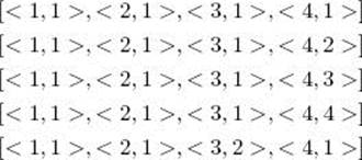
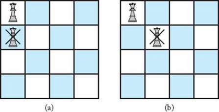
Notice that the nodes are visited according to a depth-first search in which the children of a node are visited from left to right. A simple depth-first search of a state space tree is like following every path in a maze until you reach a dead end. It does not take advantage of any signs along the way. We can make the search more efficient by looking for such signs. For example, as illustrated in Figure 5.3(a), no two queens can be in the same column. Therefore, there is no point in constructing and checking any paths in the entire branch emanating from the node containing <2, 1> in Figure 5.2. (Because we have already placed queen 1 in column 1, we cannot place queen 2 there.) This sign tells us that this node can lead to nothing but dead ends. Similarly, as illustrated in Figure 5.3(b), no two queens can be on the same diagonal. Therefore, there is no point in constructing and checking the entire branch emanating from the node containing <2, 2> in Figure 5.2.

Figure 5.2 A portion of the state space tree for the instance of the n-Queens problem in which n = 4. The ordered pair <i, j >, at each node means that the queen in the ith row is placed in the j th column. Each path from the root to a leaf is a candidate solution.

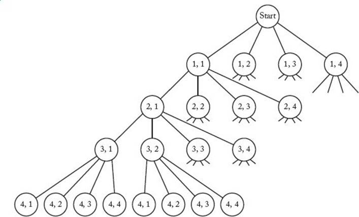
Figure 5.3 Diagram showing that if the first queen is placed in column 1, the second queen cannot be placed in column 1 (a) or column 2 (b).

Backtracking is the procedure whereby, after determining that a node can lead to nothing but dead ends, we go back (“backtrack”) to the node’s parent and proceed with the search on the next child. We call a node nonpromising if when visiting the node we determine that it cannot possibly lead to a solution. Otherwise, we call it promising. To summarize, backtracking consists of doing a depth-first search of a state space tree, checking whether each node is promising, and, if it is nonpromising, backtracking to the node’s parent. This is called pruning the state space tree, and the subtree consisting of the visited nodes is called the pruned state space tree. A general algorithm for the backtracking approach is as follows:

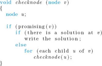
The root of the state space tree is passed to checknode at the top level. A visit to a node consists of first checking whether it is promising. If it is promising and there is a solution at the node, the solution is printed. If there is not a solution at a promising node, the children of the node are visited. The function promising is different in each application of backtracking. We call it the promising function for the algorithm. A backtracking algorithm is identical to a depth-first search, except that the children of a node are visited only when the node is promising and there is not a solution at the node. (Unlike the algorithm for the n-Queens problem, in some backtracking algorithms a solution can be found before reaching a leaf in the state space tree.) We have called the backtracking procedure checknode rather than backtrack because backtracking does not occur when the procedure is called. Rather, it occurs when we find that a node is nonpromising and proceed to the next child of the parent. A computer implementation of the recursive algorithm accomplishes backtracking by popping the activation record for a nonpromising node from the stack of activation records.

Next we use backtracking to solve the instance of the n-Queens problem when n = 4.

Example 5.1

Recall that the function promising is different for each application of backtracking. For the n-Queens problem, it must return false if a node and any of the node’s ancestors place queens in the same column or diagonal. Figure 5.4 shows a portion of the pruned state space tree produced when backtracking is used to solve the instance in which n = 4. Only the nodes checked to find the first solution are shown. Figure 5.5 shows the actual chessboards. A node is marked with a cross in Figure 5.4 if it is nonpromising. Similarly, there is a cross in a nonpromising position in Figure 5.5. The color-shaded node in Figure 5.4 is the one where the first solution is found. A walk-through of the traversal done by backtracking follows. We refer to a node by the ordered pair stored at that node. Some of the nodes contain the same ordered pair, but you can tell which node we mean by traversing the tree in Figure 5.4 while we do the walk-through.

Figure 5.4 A portion of the pruned state space tree produced when backtracking is used to solve the instance of the n-Queens problems in which n = 4. Only the nodes checked to find the first solution are shown. That solution is found at the color-shaded node. Each nonpromising node is marked with a cross.

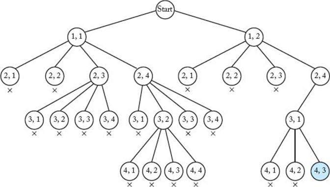
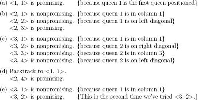
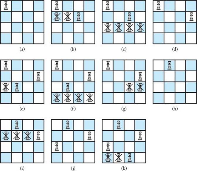
Figure 5.5 The actual chessboard positions that are tried when backtracking is used to solve the instance of the n-Queens problem in which n = 4. Each nonpromising position is marked with a cross.

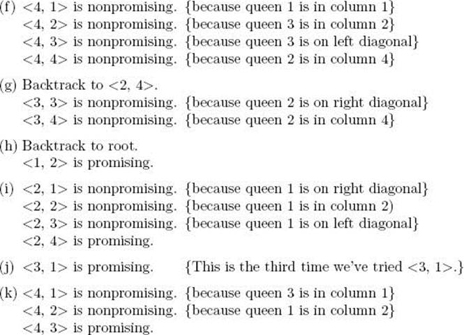
At this point the first solution has been found. It appears in Figure 5.5(k), and the node at which it is found is shaded in Figure 5.4.

Notice that a backtracking algorithm need not actually create a tree. Rather, it only needs to keep track of the values in the current branch being investigated. This is the way we implement backtracking algorithms. We say that the state space tree exists implicitly in the algorithm because it is not actually constructed.

A node count in Figure 5.4 shows that the backtracking algorithm checks 27 nodes before finding a solution. In the exercises you will show that, without backtracking, a depth-first search of the state space tree checks 155 nodes before finding that same solution.

You may have observed that there is some inefficiency in our general algorithm for backtracking (procedure checknode). That is, we check whether a node is promising after passing it to the procedure. This means that activation records for nonpromising nodes are unnecessarily placed on the stack of activation records. We could avoid this by checking whether a node is promising before passing it. A general algorithm for backtracking that does this is as follows:

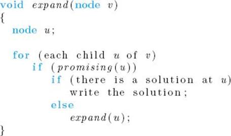
The node passed at the top level to the procedure is again the root of the tree. We call this procedure expand because we expand a promising node. A computer implementation of this algorithm accomplishes backtracking from a nonpromising node by not pushing an activation record for the node onto the stack of activation records.

In explaining algorithms in this chapter, we use the first version of the algorithm (procedure checknode) because we have found that this version typically produces algorithms that are easier to understand. The reason is that one execution of checknode consists of the steps done when visiting a single node. That is, it consists of the following steps. Determine if the node is promising. If it is promising, then if there is a solution at the node, print the solution; otherwise, visit its children. On the other hand, one execution of expand involves doing the same steps for all children of a node. After seeing the first version of an algorithm, it is not hard to write the second version.

Next we will develop backtracking algorithms for several problems, starting with the n-Queens problem. In all these problems, the state space tree contains an exponentially large or larger number of nodes. Backtracking is used to avoid unnecessary checking of nodes. Given two instances with the same value of n, a backtracking algorithm may check very few nodes for one of them but the entire state space tree for the other. This means that we will not obtain efficient time complexities for our backtracking algorithms as we did for the algorithms in the preceding chapters. Therefore, instead of the types of analyses done in those chapters, we will analyze our backtracking algorithms using the Monte Carlo technique. This technique enables us to determine whether we can expect a given backtracking algorithm to be efficient for a particular instance. The Monte Carlo technique is discussed in Section 5.3.

5.2 The n-Queens Problem

We have already discussed the goal in the n-Queens problem. The promising function must check whether two queens are in the same column or diagonal. If we let col(i) be the column where the queen in the ith row is located, then to check whether the queen in the kth row is in the same column, we need to check whether

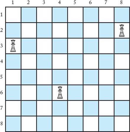
Next let’s see how to check the diagonals. Figure 5.6 illustrates the instance in which n = 8. In that figure, the queen in row 6 is being threatened in its left diagonal by the queen in row 3, and in its right diagonal by the queen in row 2. Notice that

That is, for the queen threatening from the left, the difference in the columns is the same as the difference in the rows. Furthermore,

That is, for the queen threatening from the right, the difference in the columns is the negative of the difference in the rows. These are examples of the general result that if the queen in the kth row threatens the queen in the ith row along one of its diagonals, then

Next we present the algorithm.

Figure 5.6 The queen in row 6 is being threatened in its left diagonal by the queen in row 3 and in its right diagonal by the queen in row 2.

Algorithm 5.1

The Backtracking Algorithm for the n-Queens Problem

Problem: Position n queens on a chessboard so that no two are in the same row, column, or diagonal.

Inputs: positive integer n.

Outputs: all possible ways n queens can be placed on an n × n chessboard so that no two queens threaten each other. Each output consists of an array of integers col indexed from 1 to n, where col[i] is the column where the queen in the ith row is placed.

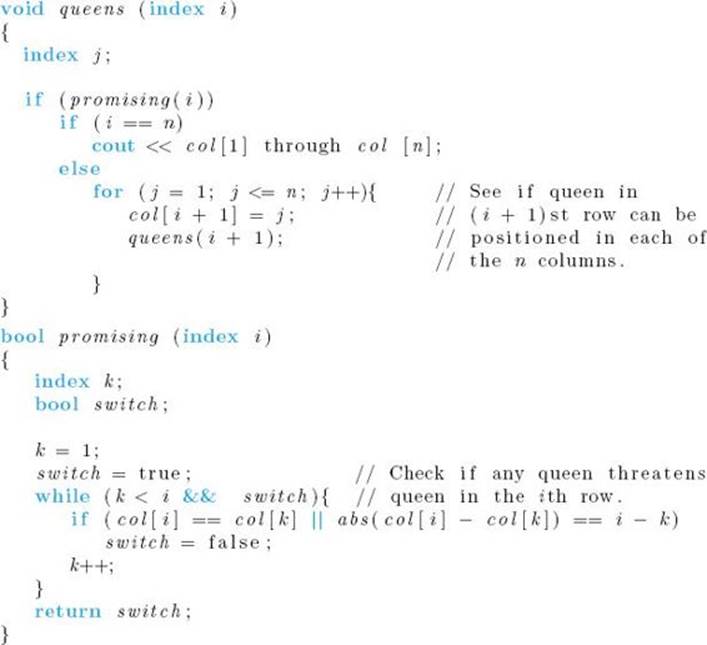
When an algorithm consists of more than one routine, we do not order the routines according to the rules of any particular programming language. Rather, we just present the main routine first. In Algorithm 5.1, that routine is queens. Following the convention discussed in Section 2.1, n and colare not inputs to the recursive routine queens. If the algorithm were implemented by defining n and col globally, the top-level call to queens would be

Algorithm 5.1 produces all solutions to the n-Queens problem because that is how we stated the problem. We stated the problem this way to eliminate the need to exit when a solution is found. This makes the algorithm less cluttered. In general, the problems in this chapter can be stated to require one, several, or all solutions. In practice, the one that is done depends on the needs of the application. Most of our algorithms are written to produce all solutions. It is a simple modification to make the algorithms stop after finding one solution.

It is difficult to analyze Algorithm 5.1 theoretically. To do this, we have to determine the number of nodes checked as a function of n, the number of queens. We can get an upper bound on the number of nodes in the pruned state space tree by counting the number of nodes in the entire state space tree. This latter tree contains 1 node at level 0, n nodes at level 1, n² nodes at level 2, … , and nⁿ nodes at level n. The total number of nodes is

This equality is obtained in Example A.4 in Appendix A. For the instance in which n = 8, the state space tree contains

This analysis is of limited value because the whole purpose of backtracking is to avoid checking many of these nodes.

Another analysis we could try is to obtain an upper bound on the number of promising nodes. To compute such a bound, we can use the fact that no two queens can ever be placed in the same column. For example, consider the instance in which n = 8. The first queen can be positioned in any of the eight columns. Once the first queen is positioned, the second can be positioned in at most seven columns; once the second is positioned, the third can he positioned in at most six columns; and so on. Therefore, there are at most

Generalizing this result to an arbitrary n, there are at most

This analysis does not give us a very good idea as to the efficiency of the algorithm for the following reasons: First, it does not take into account the diagonal check in function promising. Therefore, there could be far less promising nodes than this upper bound. Second, the total number of nodes checked includes both promising and nonpromising nodes. As we shall see, the number of nonpromising nodes can be substantially greater than the number of promising nodes.

A straightforward way to determine the efficiency of the algorithm is to actually run the algorithm on a computer and count how many nodes are checked. Table 5.1 shows the results for several values of n. The back-tracking algorithm is compared with two other algorithms for the n-Queens problem. Algorithm 1 is a depth-first search of the state space tree without backtracking. The number of nodes it checks is the number in the state space tree. Algorithm 2 uses only the fact that no two queens can be in the same row or in the same column. Algorithm 2 generates n! candidate solutions by trying the row-1 queen in each of the n columns, the row-2 queen in each of the n − 1 columns not occupied by the first queen, the row-3 queen in each of the n − 2 columns not occupied by either of the first two queens, and so on. After generating a candidate solution, it checks whether two queens threaten each other in a diagonal. Notice that the advantage of the back-tracking algorithm increases dramatically with n. When n = 4, Algorithm 1 checks less than six times as many nodes as the backtracking algorithm, and the backtracking algorithm seems slightly inferior to Algorithm 2. But when n = 14, Algorithm 1 checks almost 32 million times as many nodes as does the backtracking algorithm, and the number of candidate solutions generated by Algorithm 2 is about 230 times the number of nodes checked by backtracking. We have listed the number of promising nodes in Table 5.1 to show that many of the nodes checked can be nonpromising. This means that our second way of implementing backtracking (procedure expand, which is discussed in Section 5.1) can save a significant amount of time.

• Table 5.1 An illustration of how much checking is saved by backtracking in the n-Queens problem ∗

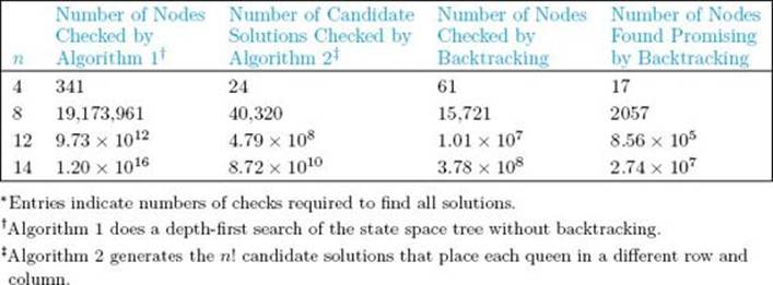
Actually running an algorithm to determine its efficiency (as was done to create Table 5.1) is not really an analysis. We did this to illustrate how much time backtracking can save. The purpose of an analysis is to determine ahead of time whether an algorithm is efficient. In the next section we show how the Monte Carlo technique can be used to estimate the efficiency of a backtracking algorithm.

Recall that in our state space tree for the n-Queens problem we use the fact that no two queens can be in the same row. Alternatively, we could create a state space tree that tries every queen in each of the n² board positions. We would backtrack in this tree whenever a queen was placed in the same row, column, or diagonal as a queen already positioned. Every node in this state space tree would have n² children, one for each board position. There would be (n²)ⁿ leaves, each representing a different candidate solution. An algorithm that backtracked in this state space tree would find no more promising nodes than our algorithm finds, but it would still be slower than ours because of the extra time needed to do a row check in function promising and because of the extra nonpromising nodes that would be investigated (that is, any node that attempted to place a queen in a row that was already occupied). In general, it is most efficient to build as much information as possible into the state space tree.

The time spent in the promising function is a consideration in any backtracking algorithm. That is, our goal is not strictly to cut down on the number of nodes checked; rather, it is to improve overall efficiency. A very time-consuming promising function could offset the advantage of checking fewer nodes. In the case of Algorithm 5.1, the promising function can be improved by keeping track of the sets of columns, of left diagonals, and of right diagonals controlled by the queens already placed. In this way, it is not necessary to check whether the queens already positioned threaten the current queen. We need only check if the current queen is being placed in a controlled column or diagonal. This improvement is investigated in the exercises.

5.3 Using a Monte Carlo Algorithm to Estimate the Efficiency of a Backtracking Algorithm

As mentioned previously, the state space tree for each of the algorithms presented in the following sections contains an exponentially large or larger number of nodes. Given two instances with the same value of n, one of them may require that very few nodes be checked, whereas the other requires that the entire state space tree be checked. If we had an estimate of how efficiently a given backtracking algorithm would process a particular instance, we could decide whether using the algorithm on that instance was reasonable. We can obtain such an estimate using a Monte Carlo algorithm.

Monte Carlo algorithms are probabilistic algorithms. By a probabilistic algorithm, we mean one in which the next instruction executed is sometimes determined at random according to some probability distribution. (Unless otherwise stated, we assume that probability distribution is the uniform distribution.) By a deterministic algorithm, we mean one in which this cannot happen. All the algorithms discussed so far have been deterministic algorithms. A Monte Carlo algorithm estimates the expected value of a random variable, defined on a sample space, from its average value on a random sample of the sample space. (See Section A.8.1 in Appendix A for a discussion of sample spaces, random samples, random variables, and expected values.) There is no guarantee that the estimate is close to the true expected value, but the probability that it is close increases as the time available to the algorithm increases.

We can use a Monte Carlo algorithm to estimate the efficiency of a backtracking algorithm for a particular instance as follows. We generate a “typical path” in the tree consisting of the nodes that would be checked given that instance, and then estimate the number of nodes in this tree from the path. The estimate is an estimate of the total number of nodes that would be checked to find all solutions. That is, it is an estimate of the number of nodes in the pruned state space tree. The following conditions must be satisfied by the algorithm in order for the technique to apply:

1. The same promising function must be used on all nodes at the same level in the state space tree.

2. Nodes at the same level in the state space tree must have the same number of children.

Notice that Algorithm 5.1 (The Backtracking Algorithm for the n-Queens Problem) satisfies these conditions.

The Monte Carlo technique requires that we randomly generate a promising child of a node according to the uniform distribution. By this we mean that a random process is used to generate the promising child. (See Section A.8.1 in Appendix A for a discussion of random processes.) When implementing the technique on a computer, we can generate only a pseudorandom promising child. The technique is as follows:

• Let m₀ be the number of promising children of the root.

• Randomly generate a promising node at level 1. Let m₁ be the number of promising children of this node.

• Randomly generate a promising child of the node obtained in the previous step. Let m₂ be the number of promising children of this node.

• Randomly generate a promising child of the node obtained in the previous step. Let m_i be the number of promising children of this node.

This process continues until no promising children are found. Because we assume that nodes at the same level in the state space tree all have the same number of children, m_i is an estimate of the average number of promising children of nodes at level i. Let

Because all t_i children of a node are checked and only the m_i promising children have children that are checked, an estimate of the total number of nodes checked by the backtracking algorithm to find all solutions is given by

A general algorithm for computing this estimate follows. In this algorithm, a variable mprod is used to represent the product m₀m₁ · · · m_i−₁ at each level.

Algorithm 5.2

Monte CarIo Estimate

Problem: Estimate the efficiency of a backtracking algorithm using a Monte Carlo algorithm.

Inputs: an instance of the problem that the backtracking algorithm solves.

Outputs: an estimate of the number of nodes in the pruned state space tree produced by the algorithm, which is the number of the nodes the algorithm will check to find all solutions to the instance.

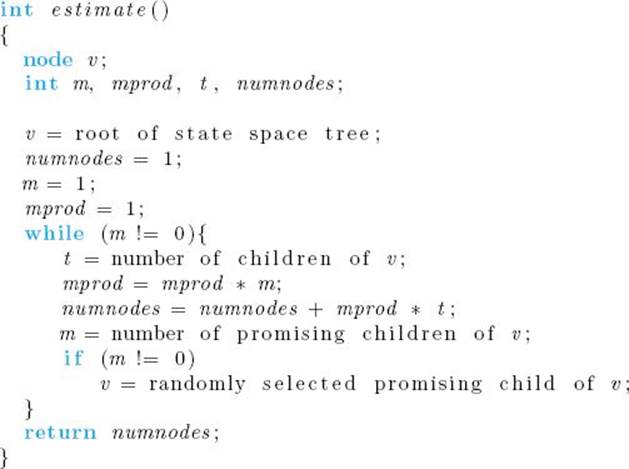
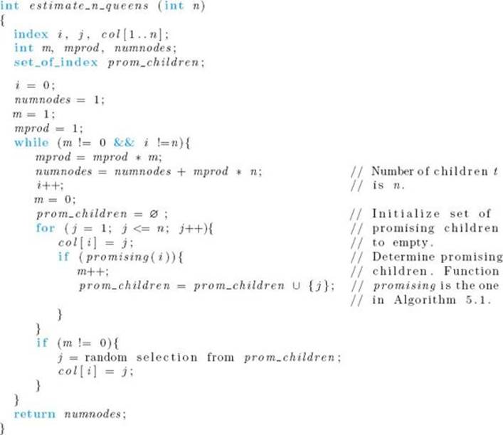
A specific version of Algorithm 5.2 for Algorithm 5.1 (The Backtracking Algorithm for the n-Queens Problem) follows. We pass n to this algorithm because n is the parameter to Algorithm 5.1.

Algorithm 5.3

Monte Carlo Estimate for Algorithm 5.1 (The Backtracking Algorithm for the n-Queens Problem)

Problem: Estimate the efficiency of Algorithm 5.1.

Inputs: positive integer n.

Outputs: an estimate of the number of nodes in the pruned state space tree produced by Algorithm 5.1, which is the number of the nodes the algorithm will check before finding all ways to position n queens on an n×n chessboard so that no two queens threaten each other.

When a Monte Carlo algorithm is used, the estimate should be run more than once, and the average of the results should be used as the actual estimate. Using standard methods from statistics, one can determine a confidence interval for the actual number of nodes checked from the results of the trials. As a rule of thumb, around 20 trials are ordinarily sufficient. We caution that although the probability of obtaining a good estimate is high when the Monte Carlo algorithm is run many times, there is never a guarantee that it is a good estimate.

The n-Queens problem has only one instance for each value of n. This is not so for most problems solved with backtracking algorithms. The estimate produced by any one application of the Monte Carlo technique is for one particular instance. As discussed before, given two instances with the same value of n, one may require that very few nodes be checked whereas the other requires that the entire state space tree be checked.

The estimate obtained using a Monte Carlo estimate is not necessarily a good indication of how many nodes will be checked before the first solution is found. To obtain only one solution, the algorithm may check a small fraction of the nodes it would check to find all solutions. For example,Figure 5.4 shows that the two branches that place the first queen in the third and fourth columns, respectively, need not be traversed to find only one solution.

5.4 The Sum-of-Subsets Problem

Recall our thief and the 0-1 Knapsack problem from Section 4.5.1. In this problem, there is a set of items the thief can steal, and each item has its own weight and profit. The thief’s knapsack will break if the total weight of the items in it exceeds W. Therefore, the goal is to maximize the total value of the stolen items while not making the total weight exceed W . Suppose here that the items all have the same profit per unit weight. Then an optimal solution for the thief would simply be a set of items that maximized the total weight, subject to the constraint that its total weight did not exceed W . The thief might first try to determine whether there was a set whose total weight equaled W, because this would be best. The problem of determining such sets is called the Sum-of-Subsets problem.

Specifically, in the Sum-of-Subsets problem, there are n positive integers (weights) w_i and a positive integer W. The goal is to find all subsets of the integers that sum to W. As mentioned earlier, we usually state our problems so as to find all solutions. For the purposes of the thief’s application, however, only one solution need be found.

Example 5.2

Suppose that n = 5, W = 21, and

Because

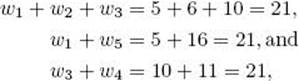
the solutions are {w₁, w₂, w₃}, {w₁, w₅}, and {w₃, w₄}.

Figure 5.7 A state space tree for instances of the Sum-of-Subsets problem in which n = 3.

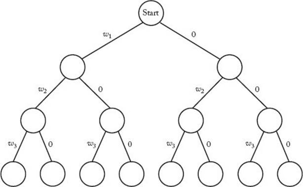
This instance can be solved by inspection. For larger values of n, a systematic approach is necessary. One approach is to create a state space tree. A possible way to structure the tree appears in Figure 5.7. For the sake of simplicity, the tree in this figure is for only three weights. We go to the left from the root to include w₁, and we go to the right to exclude w₁. Similarly, we go to the left from a node at level 1 to include w₂, and we go to the right to exclude w₂, etc. Each subset is represented by a path from the root to a leaf. When we include w_i, we write w_i on the edge where we include it. When we do not include w_i, we write 0.

Example 5.3

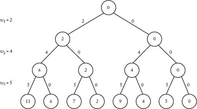
Figure 5.8 shows the state space tree for n = 3, W = 6, and

At each node, we have written the sum of the weights that have been included up to that point. Therefore, each leaf contains the sum of the weights in the subset leading to that leaf. The second leaf from the left is the only one containing a 6. Because the path to this leaf represents the subset {w1, w2}, this subset is the only solution.

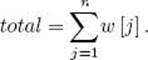
If we sort the weights in nondecreasing order before doing the search, there is an obvious sign telling us that a node is nonpromising. If the weights are sorted in this manner, then w_i₊₁ is the lightest weight remaining when we are at the ith level. Let weight be the sum of the weights that have been included up to a node at level i. If w_i₊₁ would bring the value of weight above W, then so would any other weight following it. Therefore, unless weight equals W (which means that there is a solution at the node), a node at the ith level is nonpromising if

Figure 5.8 A state space tree for the Sum-of-Subsets problem for the instance in Example 5.3. Stored at each node is the total weight included up to that node.

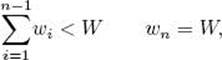
There is another, less obvious sign telling us that a node is nonpromising. If, at a given node, adding all the weights of the remaining items to weight does not make weight at least equal to W, then weight could never become equal to W by expanding beyond the node. This means that if total is the total weight of the remaining weights, a node is nonpromising if

The following example illustrates these backtracking strategies.

Example 5.4

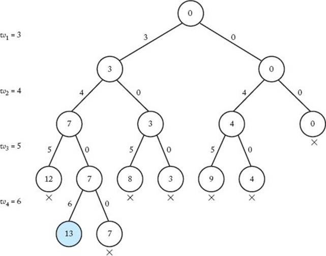
Figure 5.9 shows the pruned state space tree when backtracking is used with n = 4, W = 13, and

The only solution is found at the node shaded in color. The solution is {w₁, w₂ , w₄}. The nonpromising nodes are marked with crosses. The nodes containing 12, 8, and 9 are nonpromising because adding the next weight (6) would make the value of weight exceed W. The nodes containing 7, 3, 4, and 0 are nonpromising because there is not enough total weight remaining to bring the value of weight up to W. Notice that a leaf in the state space tree that does not contain a solution is automatically nonpromising because there are no weights remaining that could bring weight up to W. The leaf containing 7 illustrates this. There are only 15 nodes in the pruned state space tree, whereas the entire state space tree contains 31 nodes.

Figure 5.9 The pruned state space tree produced using backtracking in Example 5.4. Stored at each node is the total weight included up to that node. The only solution is found at the shaded node. Each nonpromising node is marked with a cross.

When the sum of the weights included up to a node equals W , there is a solution at that node. Therefore, we cannot get another solution by including more items. This means that if

we should print the solution and backtrack. This backtracking is provided automatically by our general procedure checknode because it never expands beyond a promising node where a solution is found. Recall that when we discussed checknode we mentioned that some backtracking algorithms sometimes find a solution before reaching a leaf in the state space tree. This is one such algorithm.

Next we present the algorithm that employs these strategies. The algorithm uses an array include. It sets include[i] to “yes” if w[i] is to be included and to “no” if it is not.

Algorithm 5.4

The Backtracking Algorithm for the Sum-of-Subsets Problem

Problem: Given n positive integers (weights) and a positive integer W, determine all combinations of the integers that sum to W.

Inputs: positive integer n, sorted (nondecreasing order) array of positive integers w indexed from 1 to n, and a positive integer W.

Outputs: all combinations of the integers that sum to W.

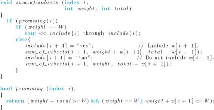
Following our usual convention, n, w, W, and include are not inputs to our routines. If these variables were defined globally, the top-level call to sum_of_subsets would be as follows:

where initially

Recall that a leaf in the state space tree that does not contain a solution is nonpromising because there are no weights left that could bring the value of weight up to W. This means that the algorithm should not need to check for the terminal condition i = n. Let’s verify that the algorithm implements this correctly. When i = n, the value of total is 0 (because there are no weights remaining). Therefore, at this point

which means that

is true only if weight ≥ W. Because we always keep weight ≤ W, we must have weight = W . Therefore, when i = n, function promising returns true only if weight = W . But in this case there is no recursive call because we found a solution. Therefore, we do not need to check for the terminal condition i = n. Notice that there is never a reference to the nonexistent array item w[n + 1] in function promising because of our assumption that the second condition in an or expression is not evaluated when the first condition is true.

The number of nodes in the state space tree searched by Algorithm 5.4 is equal to

This equality is obtained in Example A.3 in Appendix A. Given only this result, the possibility exists that the worst case could be much better than this. That is, it could be that for every instance only a small portion of the state space tree is searched. This is not the case. For each n, it is possible to construct an instance for which the algorithm visits an exponentially large number of nodes. This is true even if we want only one solution. To this end, if we take

there is only one solution {W_n}, and it will not be found until an exponentially large number of nodes are visited. As stressed before, even though the worst case is exponential, the algorithm can be efficient for many large instances. In the exercises, you are asked to write programs using the Monte Carlo technique to estimate the efficiency of Algorithm 5.4 on various instances.

Even if we state the problem so as to require only one solution, the Sum-of-Subsets problem, like the 0-1 Knapsack problem, is in the class of problems discussed in Chapter 9.

5.5 Graph Coloring

The m-Coloring problem concerns finding all ways to color an undirected graph using at most m different colors, so that no two adjacent vertices are the same color. We usually call the m-Coloring problem a unique problem for each value of m.

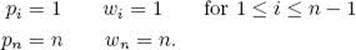
Figure 5.10 Graph for which there is no solution to the 2-Coloring problem. A solution to the 3-Coloring problem for this graph is shown in Example 5.5.

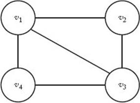
Example 5.5

Consider the graph in Figure 5.10. There is no solution to the 2-Coloring problem for this graph because, if we can use at most two different colors, there is no way to color the vertices so that no adjacent vertices are the same color. One solution to the 3-Coloring problem for this graph is as follows:

There are a total of six solutions to the 3-Coloring problem for this graph. However, the six solutions are only different in the way the colors are permuted. For example, another solution is to color v₁ color 2, v₂ and v₄ color 1, and v₃ color 3.

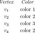
An important application of graph coloring is the coloring of maps. A graph is called planar if it can be drawn in a plane in such a way that no two edges cross each other. The graph at the bottom of Figure 5.11 is planar. However, if we were to add the edges (v₁, v₅) and (v₂, v₄) it would no longer be planar. To every map there corresponds a planar graph. Each region in the map is represented by a vertex. If one region is adjacent to another region, we join their corresponding vertices by an edge. Figure 5.11 shows a map at the top and its planar graph representation at the bottom. Them-Coloring problem for planar graphs is to determine how many ways the map can be colored, using at most m colors, so that no two adjacent regions are the same color.

A straightforward state space tree for the m-Coloring problem is one in which each possible color is tried for vertex v₁ at level 1, each possible color is tried for vertex v₂ at level 2, and so on until each possible color has been tried for vertex v_n at level n. Each path from the root to a leaf is a candidate solution. We check whether a candidate solution is a solution by determining whether any two adjacent vertices are the same color. To avoid confusion, remember in the following discussion that “node” refers to a node in the state space tree and “vertex” refers to a vertex in the graph being colored.

Figure 5.11 Map (top) and its planar graph representation (bottom).

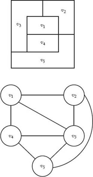
We can backtrack in this problem because a node is nonpromising if a vertex that is adjacent to the vertex being colored at the node has already been colored the color that is being used at the node. Figure 5.12 shows a portion of the pruned state space tree that results when this backtracking strategy is applied to a 3-coloring of the graph in Figure 5.10. The number in a node is the number of the color used on the vertex being colored at the node. The first solution is found at the shaded node. Nonpromising nodes are labeled with crosses. After v₁ is colored color 1, choosing color 1 forv₂ is nonpromising because v₁ is adjacent to v₂. Similarly, after v₁, v₂, and v₃ have been colored colors 1, 2, and 3, respectively, choosing color 1 for v₄ is nonpromising because v₁ is adjacent to v₄.

Figure 5.12 A portion of the pruned state space tree produced using backtracking to do a 3-coloring of the graph in Figure 5.10. The first solution is found at the shaded node. Each nonpromising node is marked with a cross.

Next we present an algorithm that solves the m-Coloring problem for all values of m. In this algorithm the graph is represented by an adjacency matrix, as was done in Section 4.1. However, because the graph is unweighted, each entry in the matrix is simply true or false depending on whether or not there is an edge between the two vertices.

Algorithm 5.5

The Backtracking Algorithm for the m-Coloring Problem

Problem: Determine all ways in which the vertices in an undirected graph can be colored, using only m colors, so that adjacent vertices are not the same color.

Inputs: positive integers n and m, and an undirected graph containing n vertices. The graph is represented by a two-dimensional array W, which has both its rows and columns indexed from 1 to n, where W [i] [j] is true if there is an edge between ith vertex and the jth vertex and false otherwise.

Outputs: all possible colorings of the graph, using at most m colors, so that no two adjacent vertices are the same color. The output for each coloring is an array vcolor indexed from 1 to n, where vcolor [i] is the color (an integer between 1 and m) assigned to the ith vertex.

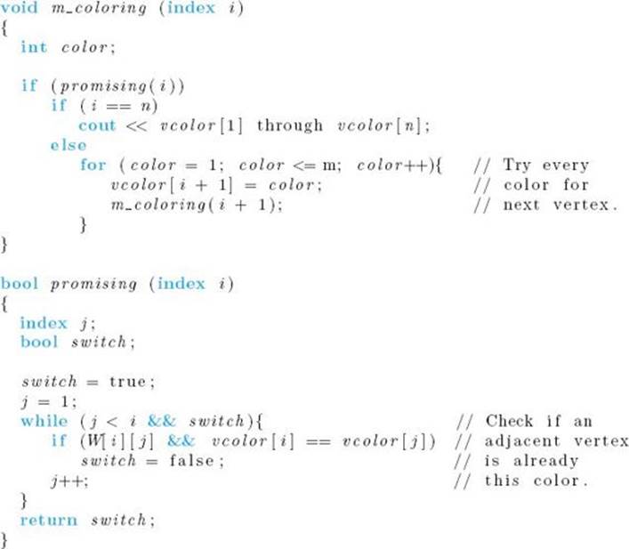
Following our usual convention, n, m, W , and vcolor are not inputs to either routine. In an implementation of the algorithm, the routines would be defined locally in a simple procedure that had n, m, and W as inputs, and vcolor defined locally. The top level call to m_coloring would be

m_coloring (0).

The number of nodes in the state space tree for this algorithm is equal to

This equality is obtained in Example A.4 in Appendix A. For a given m and n, it is possible to create an instance that checks at least an exponentially large number of nodes (in terms of n). For example, if m is only 2, and we take a graph in which v_n has an edge to every other node, and the only other edge is one between v_n−₂ and v_n−₁, then no solution exists, but almost every node in the state space tree will be visited to determine this. As with any backtracking algorithm, the algorithm can be efficient for a particular large instance. The Monte Carlo technique described in Section 5.3 is applicable to this algorithm, which means that it can be used to estimate the efficiency for a particular instance.

In the exercises, you are asked to solve the 2-Coloring problem with an algorithm whose worst-case time complexity is not exponential in n. For m ≥ 3, no one has ever developed an algorithm that is efficient in the worst case. Like the Sum-of-Subsets problem and the 0-1 Knapsack problem, them-Coloring problem for m ≥ 3 is in the class of problems discussed in Chapter 9. This is the case even if we are looking for only one m-coloring of the graph.

5.6 The Hamiltonian Circuits Problem

Recall Example 3.12, in which Nancy and Ralph were competing for the same sales position. The one who could cover all 20 cities in the sales territory the fastest was to win the job. Using the dynamic programming algorithm, with a time complexity given by

Nancy found a shortest tour in 45 seconds. Ralph tried computing all 19! tours. Because his algorithm takes over 3,800 years, it is still running. Of course, Nancy won the job. Suppose she did such a good job that the boss doubled her territory, giving her a 40-city territory. In this territory, however, not every city is connected to every other city by a road. Recall that we assumed that Nancy’s dynamic programming algorithm took 1 microsecond to process its basic operation. A quick calculation shows that it would take this algorithm

to determine a shortest tour for the 40-city territory. Because this amount of time is intolerable, Nancy must look for another algorithm. She reasons that perhaps it is too hard to find an optimal tour, so she becomes content with just finding any tour. If there were a road from every city to every other city, any permutation of cities would constitute a tour. However, recall that this is not the case in Nancy’s new territory. Therefore, her problem now is to find any tour in a graph. This problem is called the Hamiltonian Circuits problem, named after Sir William Hamilton, who suggested it. The problem can be stated for either a directed graph (the way we stated the Traveling Salesperson problem) or an undirected graph. Because it is usually stated for an undirected graph, this is the way we will state it here. As applied to Nancy’s dilemma, this means that there is a unique two-way road connecting two cities when they are connected at all.

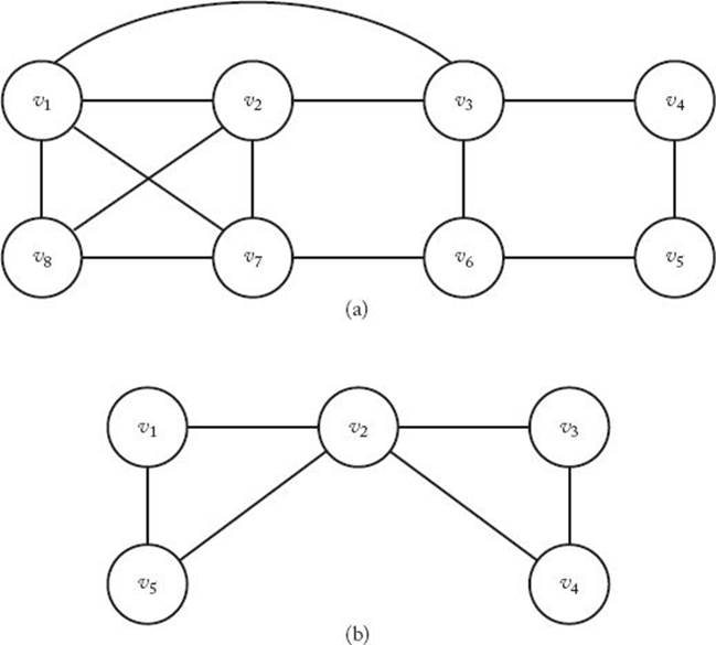
Specifically, given a connected, undirected graph, a Hamiltonian Circuit (also called a tour) is a path that starts at a given vertex, visits each vertex in the graph exactly once, and ends at the starting vertex. The graph in Figure 5.13(a) contains the Hamiltonian Circuit [v₁, v₂, v₈, v₇, v₆, v₅, v₄, v₃,v₁], but the one in Figure 5.13(b) does not contain a Hamiltonian Circuit. The Hamiltonian Circuits problem determines the Hamiltonian Circuits in a connected, undirected graph.

A state space tree for this problem is as follows. Put the starting vertex at level 0 in the tree; call it the zeroth vertex on the path. At level 1, consider each vertex other than the starting vertex as the first vertex after the starting one. At level 2, consider each of these same vertices as the second vertex, and so on. Finally, at level n − 1, consider each of these same vertices as the (n − 1)st vertex.

Figure 5.13 The graph in (a) contains the Hamiltonian Circuit [ v₁, v₂, v₈, v₇, v₆, v₅, v₄, v₃, v₂]; the graph in (b) contains no Hamiltonian Circuit.

The following considerations enable us to backtrack in this state space tree:

1. The ith vertex on the path must be adjacent to the (i − 1)st vertex on the path.

2. The (n − 1)st vertex must be adjacent to the 0th vertex (the starting one).

3. The ith vertex cannot be one of the first i − 1 vertices.

The algorithm that follows uses these considerations to backtrack. This algorithm is hard-coded to make v₁ the starting vertex.

Algorithm 5.6

The Backtracking Algorithm for the Hamiltonian Circuits Problem

Problem: Determine all Hamiltonian Circuits in a connected, undirected graph.

Inputs: positive integer n and an undirected graph containing n vertices. The graph is represented by a two-dimensional array W, which has both its rows and columns indexed from 1 to n, where W [i] [j] is true if there is an edge between the ith vertex and the jth vertex and false otherwise.

Outputs: For all paths that start at a given vertex, visit each vertex in the graph exactly once, and end up at the starting vertex. The output for each path is an array of indices vindex indexed from 0 to n − 1, where vindex[i] is the index of the ith vertex on the path. The index of the starting vertex isvindex[0].

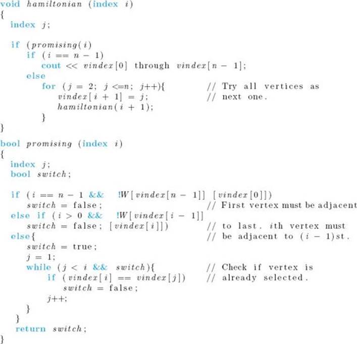
Following our convention, n, W, and vindex are not inputs to either routine. If these variables were defined globally, the top-level called to hamiltonian would be as follows:

The number of nodes in the state space tree for this algorithm is

which is much worse than exponential. This equality is obtained in Example A.4 in Appendix A. Although the following instance does not check the entire state space tree, it does check a worse-than-exponential number of nodes. Let the only edge to v₁ be one from v₂, and let all the vertices other than v₁ have edges to each other. There is no Hamiltonian Circuit for the graph, and the algorithm will check a worse-than-exponential number of nodes to learn this.

Returning to Nancy’s dilemma, the possibility exists that the backtracking algorithm (for the Hamiltonian Circuits problem) will take even longer than the dynamic programming algorithm (for the Traveling Salesperson problem) to solve her particular 40-city instance. Because the conditions for using the Monte Carlo technique are satisfied in this problem, Nancy can use that technique to estimate the efficiency for her instance. However, the Monte Carlo technique estimates the time to find all circuits. Because Nancy needs only one circuit, she can have the algorithm stop when the first circuit is found (if there is a circuit). You are encouraged to develop an instance when n = 40, estimate how quickly the algorithm should find all circuits in the instance, and run the algorithm to find one circuit. In this way you can create your own ending to the story.

Even if we want only one tour, the Hamiltonian Circuits problem is in the class of problems discussed in Chapter 9.

5.7 The 0-1 Knapsack Problem

We solved this problem using dynamic programming in Section 4.5. Here we solve it using backtracking. After that we compare the backtracking algorithm with the dynamic programming algorithm.

• 5.7.1 A Backtracking Algorithm for the 0-1 Knapsack Problem

Recall that in this problem we have a set of items, each of which has a weight and a profit. The weights and profits are positive integers. A thief plans to carry off stolen items in a knapsack, and the knapsack will break if the total weight of the items placed in it exceeds some positive integer W. The thief’s objective is to determine a set of items that maximizes the total profit under the constraint that the total weight cannot exceed W.

We can solve this problem using a state space tree exactly like the one in the Sum-of-Subsets problem (see Section 5.4). That is, we go to the left from the root to include the first item, and we go to the right to exclude it. Similarly, we go to the left from a node at level 1 to include the second item, and we go to the right to exclude it, and so on. Each path from the root to a leaf is a candidate solution.

This problem is different from the others discussed in this chapter in that it is an optimization problem. This means that we do not know if a node contains a solution until the search is over. Therefore, we back-track a little differently. If the items included up to a node have a greater total profit than the best solution so far, we change the value of the best solution so far. However, we may still find a better solution at one of the node’s descendants (by stealing more items). Therefore, for optimization problems we always visit a promising node’s children. The following is a general algorithm for backtracking in the case of optimization problems.

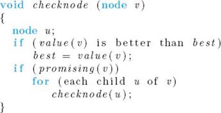
The variable best has the value of the best solution found so far, and value (v) is the value of the solution at the node. After best is initialized to a value that is worse than the value of any candidate solution, the root is passed at the top level. Notice that a node is promising only if we should expand to its children. Recall that our other algorithms also call a node promising if there is a solution at the node.

Next we apply this technique to the 0-1 Knapsack problem. First let’s look for signs telling us that a node is nonpromising. An obvious sign that a node is nonpromising is that there is no capacity left in the knapsack for more items. Therefore, if weight is the sum of the weights of the items that have been included up to some node, the node is nonpromising if

It is nonpromising even if weight equals W because, in the case of optimization problems, “promising” means that we should expand to the children.

We can use considerations from the greedy approach to find a less obvious sign. Recall that this approach failed to give an optimal solution to this problem in Section 4.5. Here we will only use greedy considerations to limit our search; we will not develop a greedy algorithm. To that end, we first order the items in nonincreasing order according to the values of p_i/w_i, where w_i and p_i are the weight and profit, respectively, of the ith item. Suppose we are trying to determine whether a particular node is promising. No matter how we choose the remaining items, we cannot obtain a higher profit than we would obtain if we were allowed to use the restrictions in the Fractional Knapsack problem from this node on. (Recall that in this problem the thief can steal any fraction of an item taken.) Therefore, we can obtain an upper bound on the profit that could be obtained by expanding beyond that node as follows. Let profit be the sum of the profits of the items included up to the node. Recall that weight is the sum of the weights of those items. We initialize variables bound and totweight to profit and weight, respectively. Next we greedily grab items, adding their profits to bound and their weights to totweight, until we get to an item that if grabbed would bring totweight above W. We grab the fraction of that item allowed by the remaining weight, and we add the value of that fraction to bound. If we are able to get only a fraction of this last weight, this node cannot lead to a profit equal to bound, but bound is still an upper bound on the profit we could achieve by expanding beyond the node. Suppose the node is at level i, and the node at level k is the one that would bring the sum of the weights above W. Then

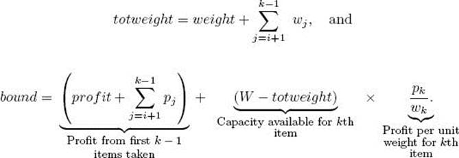
If maxprofit is the value of the profit in the best solution found so far, then a node at level i is nonpromising if

We are using greedy considerations only to obtain a bound that tells us whether we should expand beyond a node. We are not using it to greedily grab items with no opportunity to reconsider later (as is done in the greedy approach).

Before presenting the algorithm, we show an example.

Example 5.6

Suppose that n = 4, W = 16, and we have the following:

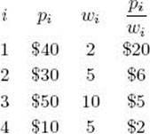
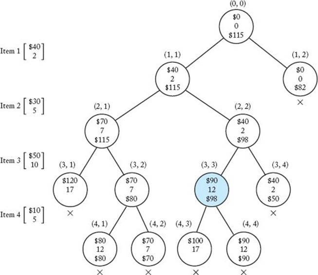
We have already ordered the items according to p_i/w_i. For simplicity, we chose values of p_i and w_i that make p_i/w_i an integer. In general, this need not be the case. Figure 5.14 shows the pruned state space tree produced by using the backtracking considerations just discussed. The total profit, total weight, and bound are specified from top to bottom at each node. These are the values of the variables profit, weight, and bound mentioned in the previous discussion. The maximum profit is found at the node shaded in color. Each node is labeled with its level and its position from the left in the tree. For example, the shaded node is labeled (3, 3) because it is at level 3 and it is the third node from the left at that level. Next we present the steps that produced the pruned tree. In these steps we refer to a node by its label.

Figure 5.14 The pruned state space tree produced using backtracking in Example 5.6. Stored at each node from top to bottom are the total profit of the items stolen up to the node, their total weight, and the bound on the total profit that could be obtained by expanding beyond the node. The optimal solution is found at the node shaded in color. Each nonpromising node is marked with a cross.

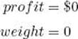
1. Set maxprofit to $0.

2. Visit node (0, 0) (the root).

(a) Compute its profit and weight.

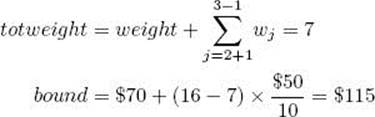
(b) Compute its bound. Because 2 + 5 + 10 = 17, and 17 > 16, the value of W , the third item would bring the sum of the weights above W. Therefore, k = 3, and we have

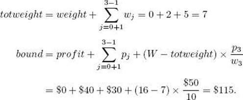
(c) Determine that the node is promising because its weight 0 is less than 16, the value of W , and its bound $115 is greater than $0, the value of maxprofit.

3. Visit node (1, 1).

(a) Compute its profit and weight.

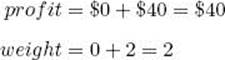
(b) Because its weight 2 is less than or equal to 16, the value of W, and its profit $40 is greater than $0, the value of maxprofit, set maxprofit to $40.

(c) Compute its bound. Because 2 + 5 + 10 = 17, and 17 > 16, the value of W , the third item would bring the sum of the weights above W. Therefore, k = 3, and we have

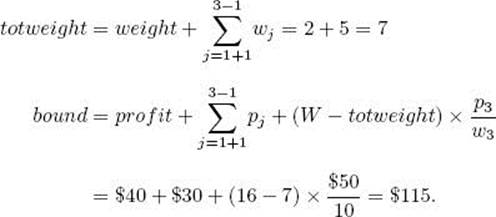
(d) Determine that the node is promising because its weight 2 is less than 16, the value of W, and its bound $115 is greater than $0, the value of maxprofit.

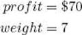
4. Visit node (2, 1).

(a) Compute its profit and weight.

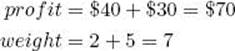
(b) Because its weight 7 is less than or equal to 16, the value of W, and its profit $70 is greater than $40, the value of maxprofit, set maxprofit to $70.

(d) Determine that the node is promising because its weight 7 is less than 16, the value of W , and its bound $115 is greater than $70, the value of maxprofit.

5. Visit node (3, 1).

(a) Compute its profit and weight.

(b) Because its weight 17 is greater than 16, the value of W, maxprofit does not change.

(d) The bound for this node is not computed, because its weight has determined it to be nonpromising.

6. Backtrack to node (2, 1).

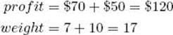
7. Visit node (3, 2).

(a) Compute its profit and weight. Because we are not including item 3,

(b) Because its profit $70 is less than or equal to $70, the value of maxprofit, maxprofit does not change.

(c) Compute its bound. The fourth weight would not bring the sum of the items above W, and there are only four items. Therefore, k = 5, and

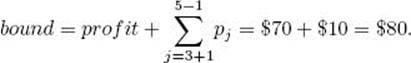
(d) Determine that the node is promising because its weight 7 is less than 16, the value of W, and its bound $80 is greater than $70, the value of maxprofit.

(From now on we leave the computations of profits, weights, and bounds as exercises. Furthermore, when maxprofit does not change, we will not mention it.)

8. Visit node (4, 1).

(a) Compute its profit and weight to be $80 and 12.

(b) Because its weight 12 is less than or equal to 16, the value of W, and its profit $80 is greater than $70, the value of maxprofit, set maxprofit to $80.

(d) Determine that it is nonpromising because its bound $80 is less than or equal to $80, the value of maxprofit. Leaves in the state space tree are automatically nonpromising because their bounds are always less than or equal to maxprofit.

9. Backtrack to node (3, 2).

10. Visit node (4, 2).

(a) Compute its profit and weight to be $70 and 7.

(b) Compute its bound to be $70.

(c) Determine that the node is nonpromising because its bound $70 is less than or equal to $80, the value of maxprofit.

11. Backtrack to node (1, 1).

12. Visit node (2, 2).

(a) Compute its profit and weight to be $40 and 2.

(b) Compute its bound to be $98.

(c) Determine that it is promising because its weight 2 is less than 16, the value of W , and its bound $98 is greater than $80, the value of maxprofit.

13. Visit node (3, 3).

(a) Compute its profit and weight to be $90 and 12.

(b) Because its weight 12 is less than or equal to 16, the value of W , and its profit $90 is greater than $80, the value of maxprofit, set maxprofit to $90.

(d) Determine that it is promising because its weight 12 is less than 16, the value of W , and its bound $98 is greater than $90, the value of maxprofit.

14. Visit node (4, 3).

(a) Compute its profit and weight to be $100 and 17.

(b) Determine that it is nonpromising because its weight 17 is greater than or equal to 16, the value of W .

15. Backtrack to node (3, 3).

16. Visit node (4, 4).

(a) Compute its profit and weight to be $90 and 12.

(b) Compute its bound to be $90.

17. Backtrack to node (2, 2).

18. Visit node (3, 4).

(a) Compute its profit and weight to be $40 and 2.

(b) Compute its bound to be $50.

(c) Determine that the node is nonpromising because its bound $50 is less than or equal to $90, the value of maxprofit.

19. Backtrack to root.

20. Visit node (1, 2).

(a) Compute its profit and weight to be $0 and 0.

(b) Compute its bound to be $82.

(c) Determine that the node is nonpromising because its bound $82 is less than or equal to $90, the value of maxprofit.

21. Backtrack to root.

(a) Root has no more children. We are done.

There are only 13 nodes in the pruned state space tree, whereas the entire state space tree has 31 nodes.

Next we present the algorithm. Because this is an optimization problem, we have the added task of keeping track of the current best set of items and the total value of their profits. We do this in an array bestset and a variable maxprofit. Unlike the other problems in this chapter, we state this problem so as to find just one optimal solution.

Algorithm 5.7

The Backtracking Algorithm for the 0-1 Knapsack ProbIem

Problem: Let n items be given, where each item has a weight and a profit. The weights and profits are positive integers. Furthermore, let a positive integer W be given. Determine a set of items with maximum total profit, under the constraint that the sum of their weights cannot exceed W .

Inputs: Positive integers n and W ; arrays w and p, each indexed from 1 to n, and each containing positive integers sorted in nonincreasing order according to the values of p [i] /w [i].

Outputs: an array bestset indexed from 1 to n, where the values of bestset[i] is “yes” if the ith item is included in the optimal set and is “no” otherwise; an integer maxprofit that is the maximum profit.

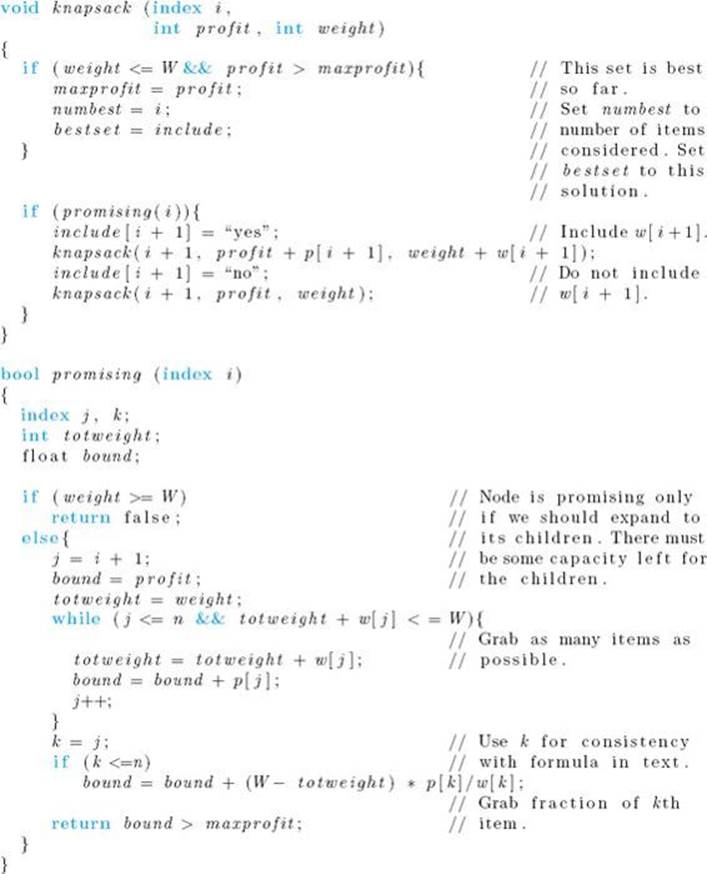
Following our usual convention, n, w, p, W , maxprofit, include, bestset, and numbest are not inputs to either routine. If these variables were defined globally, the following code would produce the maximum profit and a set that has that profit:

Recall that leaves in the state space tree are automatically nonpromising because their bounds cannot be greater than maxprofit. Therefore, we should not need a check for the terminal condition that i = n in function promising. Let’s confirm that our algorithm does not need to do this check. If i =n, bound does not change from its initial value profit. Because profit is less than or equal to maxprofit, the expression bound>maxprofit is false, which means that function promising returns false.

Our upper bound does not change value as we repeatedly proceed to the left in the state space tree until we reach the node at level k. (This can he seen by looking again at the first few steps in Example 5.6.) Therefore, each time a value of k is established, we can save its value and proceed to the left without calling function promising until we reach the node at the (k − 1)st level. We know that the left child of this node is nonpromising because including the kth item would bring the value of weight above W . Therefore, we proceed only to the right from this node. It is only after a move to the right that we need to call function promising and determine a new value of k. In the exercises you are asked to write this improvement.

The state space tree in the 0-1 Knapsack problem is the same as that in the Sum-of-Subsets problem. As shown in Section 5.4, the number of nodes in that tree is

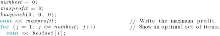
Algorithm 5.7 checks all nodes in the state space tree for the following instances. For a given n, let W = n, and

The optimal solution is to take only the nth item, and this solution will not be found until we go all the way to the right to a depth of n − 1 and then go left. Before the optimal solution is found, however, every nonleaf will be found to be promising, which means that all nodes in the state space tree will be checked. Because the Monte Carlo technique applies in this problem, it can be used to estimate the efficiency of the algorithm for a particular instance.

• 5.7.2 Comparing the Dynamic Programming Algorithm and the Backtracking Algorithm for the 0-1 Knapsack Problem

Recall from Section 4.5 that the worst-case number of entries that is computed by the dynamic programming algorithm for the 0-1 Knapsack problem is in O (minimum (2ⁿ, nW)). In the worst case, the backtracking algorithm checks Θ (2ⁿ) nodes. Owing to the additional bound of nW , it may appear that the dynamic programming algorithm is superior. However, in backtracking algorithms the worst case gives little insight into how much checking is usually saved by backtracking. With so many considerations, it is difficult to analyze theoretically the relative efficiencies of the two algorithms. In cases such as this, the algorithms can be compared by running them on many sample instances and seeing which algorithm usually performs better. Horowitz and Sahni (1978) did this and found that the back-tracking algorithm is usually more efficient than the dynamic programming algorithm.

Horowitz and Sahni (1974) coupled the divide-and-conquer approach with the dynamic programming approach to develop an algorithm for the 0-1 Knapsack problem that is O (2ⁿ^/2) in the worst case. They showed that this algorithm is usually more efficient than the backtracking algorithm.

EXERCISES

Sections 5.1 and 5.2

1. Show the first two solutions to the n-Queens problem for n = 6 and n = 7 (two solutions for each) using the Backtracking algorithm.

2. Apply the Backtracking algorithm for the n-Queens problem (Algorithm 5.1) to the problem instance in which n = 8, and show the actions step by step. Draw the pruned state space tree produced by this algorithm up to the point where the first solution is found.

3. Write a backtracking algorithm for the n-Queens problem that uses a version of procedure expand instead of a version of procedure checknode.

4. Write an algorithm that takes an integer n as input and determines the total number of solutions to the n-Queens problem.

5. Show that, without backtracking, 155 nodes must be checked before the first solution to the n = 4 instance of the n-Queens problem is found (in contrast to the 27 nodes in Figure 5.4).

6. Implement the Backtracking algorithm for the n-Queens problem (Algorithm 5.1) on your system, and run it on problem instances in which n = 4, 8, 10, and 12.

7. Improve the Backtracking algorithm for the n-Queens problem (Algorithm 5.1) by having the promising function keep track of the set of columns, of left diagonals, and of right diagonals controlled by the queens already placed.

8. Modify the Backtracking algorithm for the n-Queens problem (Algorithm 5.1) so that, instead of generating all possible solutions, it finds only a single solution.

9. Suppose we have a solution to the n-Queens problem instance in which n = 4. Can we extend this solution to find a solution to the problem instance in which n = 5? Can we then use the solutions for n = 4 and n = 5 to construct a solution to the instance in which n = 6 and continue this dynamic programming approach to find a solution to any instance in which n > 4? Justify your answer.

10. Find at least two instances of the n-Queens problem that have no solutions.

Section 5.3

11. Implement algorithm 5.3 (Monte Carlo estimate for the Backtracking algorithm for the n-Queens problem) on your system, run it 20 times on the problem instance in which n = 8, and find the average of the 20 estimates.

12. Modify the Backtracking algorithm for the n-Queens problem (Algorithm 5.1) so that it finds the number of nodes checked for an instance of a problem, run it on the problem instance in which n = 8, and compare the result against the average of Exercise 9.

Section 5.4

13. Use the Backtracking algorithm for the Sum-of-Subsets problem (Algorithm 5.4) to find all combinations of the following numbers that sum to W = 52:

Show the actions step by step.

14. Implement the Backtracking algorithm for the Sum-of-Subsets problem (Algorithm 5.4) on your system, and run it on the problem instance of Exercise 11.

15. Write a backtracking algorithm for the Sum-of-Subsets problem that does not sort the weights in advance. Compare the performance of this algorithm with that of Algorithm 5.4.

16. Modify the Backtracking algorithm for the Sum-of-Subsets problem (Algorithm 5.4) so that, instead of generating all possible solutions, it finds only a single solution. How does this algorithm perform with respect to Algorithm 5.4?

17. Use the Monte Carlo technique to estimate the efficiency of the Backtracking algorithm for the Sum-of-Subsets problem (Algorithm 5.4).

Section 5.5

18. Use the Backtracking algorithm for the m-Coloring problem (Algorithm 5.5) to find all possible colorings of the graph below using the three colors red, green, and white. Show the actions step by step.

19. Suppose that to color a graph properly we choose a starting vertex and a color to color as many vertices as possible. Then we select a new color and a new uncolored vertex to color as many more vertices as possible. We repeat this process until all the vertices of the graph are colored or all the colors are exhausted. Write an algorithm for this greedy approach to color a graph of n vertices. Analyze this algorithm and show the results using order notation.

20. Use the algorithm of Exercise 17 to color the graph of Exercise 16.

21. Suppose we are interested in minimizing the number of colors used in coloring a graph. Does the greedy approach of Exercise 17 guarantee an optimal solution? Justify your answer.

22. Construct a connected graph containing n vertices for which the 3-Coloring Backtracking algorithm will take exponential time to discover that the graph is not 3-colorable.

23. Compare the performance of the Backtracking algorithm for the m-Coloring problem (Algorithm 5.5) and the greedy algorithm of Exercise 17. Considering the result(s) of the comparison and your answer to Exercise 19, why might one be interested in using an algorithm based on the greedy approach?

24. Write an algorithm for the 2-Coloring problem whose time complexity is not worst-case exponential in n.

25. List some of the practical applications that are representable in terms of the m-Coloring problem.

Section 5.6

26. Use the Backtracking algorithm for the Hamiltonian Circuits problem (Algorithm 5.6) to find all possible Hamiltonian Circuits of the following graph.

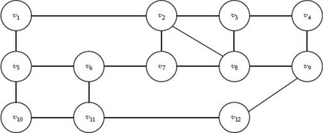
Show the actions step by step.

27. Implement the Backtracking algorithm for the Hamiltonian Circuits problem (Algorithm 5.6) on your system, and run it on the problem instance of Exercise 26.

28. Change the starting vertex in the Backtracking algorithm for the Hamiltonian Circuits problem (Algorithm 5.6) in Exercise 27 and compare its performance with that of Algorithm 5.6.

29. Modify the Backtracking algorithm for the Hamiltonian Circuits problem (Algorithm 5.6) so that, instead of generating all possible solutions, it finds only a single solution. How does this algorithm perform with respect to Algorithm 5.6?

30. Analyze the Backtracking algorithm for the Hamiltonian Circuits problem (Algorithm 5.6) and show the worst-case complexity using order notation.

31. Use the Monte Carlo Technique to estimate the efficiency of the Backtracking algorithm for the Hamiltonian Circuits problem (Algorithm 5.6).

Section 5.7

32. Compute the remaining values and bounds after visiting node (4, 1) in Example 5.6 (Section 5.7.1).

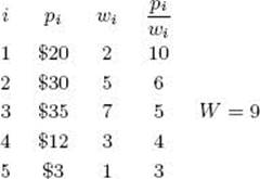
33. Use the Backtracking algorithm for the 0-1 Knapsack problem (Algorithm 5.7) to maximize the profit for the following problem instance. Show the actions step by step.

34. Implement the Backtracking algorithm for the 0-1 Knapsack problem (Algorithm 5.7) on your system, and run it on the problem instance of Exercise 30.

35. Implement the dynamic programming algorithm for the 0-1 Knapsack problem (see Section 4.5.3) and compare the performance of this algorithm with the Backtracking algorithm for the 0-1 Knapsack problem (Algorithm 5.7) using large instances of the problem.

36. Improve the Backtracking algorithm for the 0-1 Knapsack problem (Algorithm 5.7) by calling the promising function after only a move to the right.

37. Use the Monte Carlo technique to estimate the efficiency of the Backtracking algorithm for the 0-1 Knapsack problem (Algorithm 5.7).

Additional Exercises

38. List three more applications of backtracking.

39. Modify the Backtracking algorithm for the n-Queens problem (Algorithm 5.1) so that it produces only the solutions that are invariant under reflections or rotations.

40. Given an n × n × n cube containing n³ cells, we are to place n queens in the cube so that no two queens challenge each other (so that no two queens are in the same row, column, or diagonal). Can the n-Queens algorithm (Algorithm 5.1) be extended to solve this problem? If so, write the algorithm and implement it on your system to solve problem instances in which n = 4 and n = 8.

41. Modify the Backtracking algorithm for the Sum-of-Subsets (Algorithm 5.4) to produce the solutions in a variable-length list.

42. Explain how we can use the Backtracking algorithm for the m-Coloring problem (Algorithm 5.5) to color the edges of the graph of Exercise 16 using the same three colors so that edges with a common end receive different colors.

43. Modify the Backtracking algorithm for the Hamiltonian Circuits problem (Algorithm 5.6) so that it finds a Hamiltonian Circuit with minimum cost for a weighted graph. How does your algorithm perform?

44. Modify the Backtracking algorithm for the 0-1 Knapsack problem (Algorithm 5.7) to produce a solution in a variable-length list.