Foundations of Algorithms (2015)
Chapter 7 Introduction to Computational Complexity: The Sorting Problem

We presented a quadratic-time sorting algorithm (Exchange Sort) in Section 1.1. If computer scientists had been content with this sorting algorithm, many applications would now be running significantly slower and others would not be possible at all. Recall from Table 1.4 that it would take years to sort 1 billion keys using a quadratic-time algorithm. More efficient sorting algorithms have been developed. In particular, in Section 2.2 we saw Mergesort, which is Θ (n lg n) in the worst case. Although this algorithm could not sort 1 billion items so quickly that the time would be imperceptible to a human, Table 1.4 shows that it could sort the items in an amount of time that would be tolerable in an offline application. Suppose someone wanted 1 billion items to be sorted almost immediately in an online application. That person might labor for many hours or even many years trying to develop a linear-time or better sorting algorithm. Wouldn’t that individual be distraught to learn, after devoting a lifetime of work to this effort, that such an algorithm was not possible? There are two approaches to attacking a problem. One is to try to develop a more efficient algorithm for the problem. The other is to try to prove that a more efficient algorithm is not possible. Once we have such a proof, we know that we should quit trying to obtain a faster algorithm. As we shall see, for a large class of sorting algorithms, we have proven that an algorithm better than Θ (n lg n) is not possible.
7.1 Computational Complexity
The preceding chapters were concerned with developing and analyzing algorithms for problems. We often used different approaches to solve the same problem with the hope of finding increasingly efficient algorithms for the problem. When we analyze a specific algorithm, we determine its time (or memory) complexity or the order of its time (or memory) complexity. We do not analyze the problem that the algorithm solves. For example, when we analyzed Algorithm 1.4 (Matrix Multiplication), we found that its time complexity was n3. However, this does not mean that the problem of matrix multiplication requires a Θ (n3) algorithm. The function n3 is a property of that one algorithm; it is not necessarily a property of the problem of matrix multiplication. In Section 2.5 we developed Strassen’s matrix multiplication algorithm with a time complexity in Θ (n2.81). . Furthermore, we mentioned that a Θ (n2.38) variation of the algorithm has been developed. An important question is whether it is possible to find an even more efficient algorithm.
Computational complexity, which is a field that runs hand-in-hand with algorithm design and analysis, is the study of all possible algorithms that can solve a given problem. A computational complexity analysis tries to determine a lower bound on the efficiency of all algorithms for a given problem. At the end of Section 2.5, we mentioned that it has been proven that the problem of matrix multiplication requires an algorithm whose time complexity is in Ω (n2). It was a computational complexity analysis that determined this. We state this result by saying that a lower bound for the problem of matrix multiplication is Ω (n2). This does not mean that it must algorithm for matrix multiplication. It means only that is impossible to create one that is better than Θ (n2). Because our best algorithm is Θ (n2.38) and our lower bound is Ω (n2) , it is worthwhile to continue investigating the problem. The investigation can proceed in two directions. On one hand, we can try to find a more efficient algorithm using algorithm design methodology, while on the other hand we can try to obtain a greater lower bound using computational complexity analysis. Perhaps someday we will develop an algorithm that is better than Θ (n2.38), or perhaps someday we will prove that there is a lower bound greater than Ω (n2). In general, our goal for a given problem is to determine a lower of Ω (f (n)) and develop a Θ (f (n)) algorithm for the problem. Once we have done this, we know that, except for improving the constant, we cannot improve on the algorithm any further.
Some authors use the term “computational complexity analysis” to include both algorithm and problem analysis. Thoughout this text, when we refer to computational complexity analysis, we mean just problem analysis.
We introduce computational complexity analysis by studying the Sorting problem. There are two reasons for choosing this problem. First, quite a few algorithms have been devised that solve the problem. By studying and comparing these algorithms, we can gain insight into how to choose among several algorithms for the same problem and how to improve a given algorithm. Second, the problem of sorting is one of the few problems for which we have been successful in developing algorithms whose time complexities are about as good as our lower bound. That is, for a large class of sorting algorithms, we have determined a lower bound of Ω (n lg n) and we have developed Ω (n lg n) algorithms. Therefore, we can say that we have solved the Sorting problem as far as this class of algorithms is concerned.
The class of sorting algorithms for which we have obtained algorithms about as good as our lower bound includes all algorithms that sort only by comparison of keys. As discussed at the beginning of Chapter 1, the word “key” is used because records obtain a unique identifier, called key, that is an element of an ordered set. Given that records are arranged in some arbitrary sequence, the sorting task is to rearrange them so that they are in order according to the values of the keys. In our algorithms, the keys are stored in an array, and we do not refer to the nonkey fields. However, it is assumed that these fields are rearranged along with the key. Algorithms that sort only by comparisons of keys can compare two keys to determine which is larger, and can copy keys, but cannot do other operations on them. The sorting algorithms we have encountered so far (Algorithms 1.3, 2.4, and 2.6) fall into this class.
In Sections 7.2 through 7.8, we discuss algorithms that sort only by comparisons of keys. Specifically, Section 7.2 discusses Insertion Sort and Selection Sort, two of the most efficient quadratic-time sorting algorithms. In Section 7.3 we show that, as long as we limit ourselves to a restriction in Insertion Sort and Selection Sort, we cannot improve on quadratic time. Sections 7.4 and 7.5 revisit our Θ (n lg n) sorting algorithms, Mergesort and Quicksort. Section 7.6 presents another Θ (n lg n) sorting algorithm, Heapsort. In Section 7.7 we compare our three Θ (n lg n) sorting algorithms. Section 7.8 shows the proof that Ω (n lg n) is a lower bound for algorithms that sort by comparing keys. In Section 7.9 we discuss Radix Sort, which is a sorting algorithm that does not sort by comparing keys.
We analyze the algorithms in terms of both the number of comparisons of keys and the number of assignments of records. For example, in Algorithm 1.3 (Exchange Sort), the exchange of S [i] and S [j] can be implemented as follows:
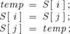
This means that three assignments of records are done to accomplish one exchange. We analyze the number of assignments of records because, when the records are large, the time taken to assign a record is quite costly. We also analyze how much extra space the algorithms require besides the space needed to store the input. When the extra space is a constant (that is, when it does not increase with n, the number of keys to be sorted), the algorithm is called an in-place sort. Finally, we assume that we are always sorting in nondecreasing order.
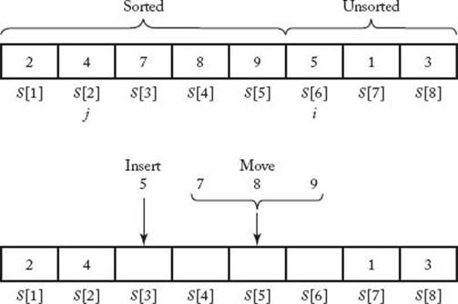
Figure 7.1 An example illustrating what Insertion Sort does when i = 6 and j = 2 (top). The array before inserting, and (bottom) the insertion step.
7.2 Insertion Sort and Selection Sort
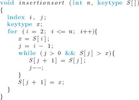
An insertion sort algorithm is one that sorts by inserting records in an existing sorted array. An example of a simple insertion sort is as follows. Assume that the keys in the first i − 1 array slots are sorted. Let x be the value of the key in the ith slot. Compare x in sequence with the key in the (i − 1)st slot, the one in the (i − 2)nd slot, etc., until a key is found that is smaller than x. Let j be the slot where that key is located. Move the keys in slots j +1 through i − 1 to slots j +2 through i, and insert x in the (j + 1)st slot. Repeat this process for i = 2 through i = n. Figure 7.1 illustrates this sort. An algorithm for this sort follows:
![]() Algorithm 7.1
Algorithm 7.1
Insertion Sort
Problem: Sort n keys in nondecreasing order.
Inputs: positive integer n; array of keys of keys S indexed from 1 to n.
Outputs: the array S containing the keys in nondecreasing order.
Analysis of Algorithm 7.1
![]() Worst-Case Time Complexity Analysis of Number of Comparisons of Keys (Insertion Sort)
Worst-Case Time Complexity Analysis of Number of Comparisons of Keys (Insertion Sort)
Basic operation: the comparison of S [j] with x.
Input size: n, the number of keys to be sorted.
For a given i, the comparison of S [j] with x is done most often when the while loop is exited because j becomes equal to 0. Assuming the second condition in an && expression is not evaluated when the first condition is false, the comparison of S [j] with x is not done when j is 0. Therefore, this comparison is done at most i−1 times for a given i. Because i ranges in value from 2 to n, the total number of comparisons is at most
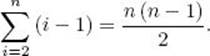
It is left as an exercise to show that, if the keys are originally in nonincreasing order in the array, this bound is achieved. Therefore,
![]()
Analysis of Algorithm 7.1
![]() Average-Case Time Complexity Analysis of Number of Comparisons of Keys (Insertion Sort)
Average-Case Time Complexity Analysis of Number of Comparisons of Keys (Insertion Sort)
For a given i, there are i slots in which x can be inserted. That is, x can stay in the ith slot, go in the (i − 1)st slot, go in the (i − 2)nd slot, etc. Because we have not previously inspected x or used it in the algorithm, we have no reason to believe that it is more likely to be inserted in any one slot than in any other. Therefore, we assign equal probabilities to each of the first i slots. This means that each slot has the probability 1/i. The following list shows the number of comparisons done when x is inserted in each slot.
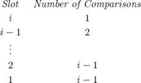
The reason the number of comparisons is i−1 and not i when x is inserted in the first slot is that the first condition in the expression controlling the while loop is false when j = 0, which means that the second condition is not evaluated. For a given i, the average number of comparisons needed to insert x is
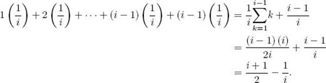
Therefore, the average number of comparisons needed to sort the array is
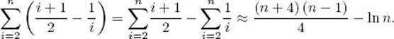
The last equality is obtained using the results of Examples A.1 and A.9 in Appendix A and doing some algebraic manipulations. We have shown that
![]()
Next we analyze the extra space usage.
Analysis of Algorithm 7.1
![]() Analysis of Extra Space Usage (Insertion Sort)
Analysis of Extra Space Usage (Insertion Sort)
The only space usage that increases with n is the size of the input array S. Therefore, the algorithm is an in-place sort, and the extra space is in Θ (1).
In the exercises, you are asked to show that the worst-case and average-case time complexities for the number of assignments of records done by Insertion Sort are given by
![]()
Next we compare Insertion Sort with the other quadratic-time algorithm encountered in this text—namely, Exchange Sort (Algorithm 1.3). Recall that the every-case time complexity of the number of comparisons of keys in Exchange Sort is given by
![]()
In the exercises, you are asked to show that the worst-case and average-case time complexities for the number of assignments of records done by Exchange Sort are given by
![]()
Clearly, Exchange Sort is an in-place sort.
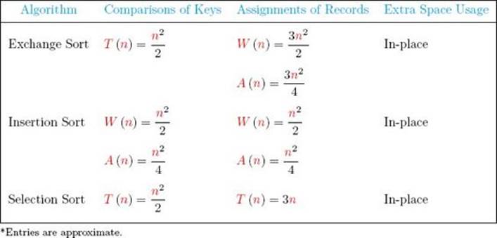
Table 7.1 summarizes our results concerning Exchange Sort and Insertion Sort. We see from this table that in terms of comparisons of keys, Insertion Sort always performs at least as well as Exchange Sort and, on the average, performs better. In terms of assignments of records, Insertion Sort performs better both in the worst-case and on the average. Because both are in-place sorts, Insertion Sort is the better algorithm. Notice that another algorithm, Selection Sort, is also included in Table 7.1. This algorithm is a slight modification of Exchange Sort and removes one of the disadvantages of Exchange Sort. We present it next.
• Table 7.1 Analysis summary for Exchange Sort, Insertion Sort, and Selection Sort
![]() Algorithm 7.2
Algorithm 7.2
Selection Sort
Problem: Sort n keys in nondecreasing order.
Inputs: positive integer n; array of keys S indexed from 1 to n.
Outputs: the array S containing the keys in nondecreasing order.
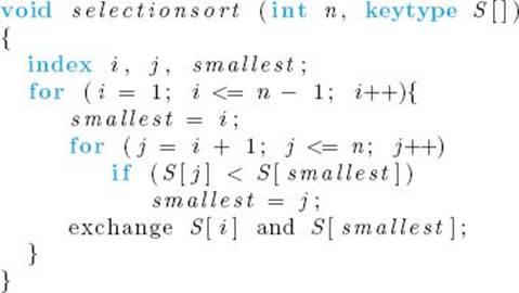
Clearly, this algorithm has the same time complexity as Exchange Sort in terms of comparisons of keys. However, the assignments of records are significantly different. Instead of exchanging S [i] and S [j] every time S [j] is found to be smaller than S [i], as Exchange Sort does (see Algorithm 1.3), Selection Sort simply keeps track of the index of the current smallest key among the keys in the ith through the nth slots. After determining that record, it exchanges it with the record in the ith slot. In this way, the smallest key is placed in the first slot after the first pass through the for-i loop, the second smallest key is put in the second slot after the second pass, and so on. The result is the same as that of Exchange Sort. However, by doing only one exchange at the bottom of the for-i loop, we have made the number of exchanges exactly n − 1. Because three assignments are needed to do an exchange, the every-case time complexity of the number of assignments of records done by Selection Sort is given by
![]()
Recall that the average-case number of assignments of records for Exchange Sort is about 3n2/4. Therefore, on the average, we’ve replaced quadratic time with linear time. Exchange Sort sometimes does better than Selection Sort. For example, if the records are already sorted, Exchange Sort does no assignments of records.
How does Selection Sort compare with Insertion Sort? Look again at Table 7.1. In terms of comparisons of keys, Insertion Sort always performs at least as well as Selection Sort and, on the average, performs better. However, Selection Sort’s time complexity in terms of assignments of records is linear whereas Insertion Sort’s is quadratic. Recall that linear time is much faster than quadratic time when n is large. Therefore, if n is large and the records are big (so that the time to assign a record is costly), Selection Sort should perform better.
Any sorting algorithm that selects records in order and puts them in their proper positions is called a selection sort. This means that Exchange Sort is also a selection sort. Another selection sort, called Heapsort, is presented in Section 7.6. Algorithm 7.2, however, has been honored with the name “Selection Sort.”
The purpose of comparing Exchange Sort, Insertion Sort, and Selection Sort was to introduce a complete comparison of sorting algorithms as simply as possible. In practice, none of these algorithms is practical for extremely large instances because all of them are quadratic-time in both the average case and the worst case. Next we show that as long as we limit ourselves to algorithms in the same class as these three algorithms, it is not possible to improve on quadratic time as far as comparisons of keys are concerned.
7.3 Lower Bounds for Algorithms that Remove at Most One Inversion per Comparison
After each comparison, Insertion Sort either does nothing or moves the key in the jth slot to the (j + 1)st slot. By moving the key in the jth slot up one slot, we have remedied the fact that x should come before that key. However, this is all that we have accomplished. We show that all sorting algorithms that sort only by comparisons of keys, and accomplish such a limited amount of rearranging after each comparison, require at least quadratic time. We obtain our results under the assumption that the keys to be sorted are distinct. Clearly, the worst-case bound still holds true with this restriction removed because a lower bound on the worst-case performance of inputs from some subsets of inputs is also a lower bound when all inputs are considered.
In general, we are concerned with sorting n distinct keys that come from any ordered set. However, without loss of generality, we can assume that the keys to be sorted are simply the positive integers 1, 2, …, n, because we can substitute 1 for the smallest key, 2 for the second smallest, and so on. For example, suppose we have the alpha input [Ralph, Clyde, Dave]. We can associate 1 with Clyde, 2 with Dave, and 3 with Ralph to obtain the equivalent input [3, 1, 2]. Any algorithm that sorts these integers only by comparisons of keys would have to do the same number of comparisons to sort the three names.
A permutation of the first n positive integers can be thought of as an ordering of those integers. Because there are n! permutations of the first n positive integers (see Section A.7), there are n! different orderings of those integers. For example, the following six permutations are all the orderings of the first three positive integers:
![]()
This means that there are n! different inputs (to a sorting algorithm) containing n distinct keys. These six permutations are the different inputs of size 3.
We denote a permutation by [k1, k2, … , kn]. That is, ki is the integer at the ith position. For the permutation [3, 1, 2], for example,
![]()
An inversion in a permutation is a pair
![]()
For example, the permutation [3, 2, 4, 1, 6, 5] contains the inversions (3, 2), (3, 1), (2, 1), (4, 1), and (6, 5). Clearly, a permutation contains no inversions if and only if it is the sorted ordering [1, 2, … , n]. This means that the task of sorting n distinct keys is the removal of all inversions in permutation. We now state the main result of this section.
![]() Theorem 7.1
Theorem 7.1
Any algorithm that sorts n distinct keys only by comparisons of keys and removes at most one inversion after each comparison must in the worst case do at least
![]()
and, on the average, do at least
![]()
Proof: To establish the result for the worst case, we need only show that there is a permutation with n (n − 1) /2 inversions, because when that permutation is the input, the algorithm will have to remove that many inversions and therefore do at least that many comparisons. Showing that [n, n − 1, … , 2, 1] is such a permutation is left as an exercise.
To establish the result for the average case, we pair the permutation [kn, kn−1, … , k1] with the permutation [k1, k2, … , kn]. This permutation is called the transpose of the original permutation. For example, the transpose of [3, 2, 4, 1, 5] is [5, 1, 4, 2, 3]. It is not hard to see that if n > 1, each permutation has a unique transpose that is distinct from the permutation itself. Let
r and s be integers between 1 and n such that s > r.
Given a permutation, the pair (s, r) is an inversion in either the permutation or its transpose but not in both. Showing that there are n (n − 1) /2 such pairs of integers between 1 and n is left as an exercise. This means that a permutation and its transpose have exactly n (n − 1) /2 inversions between them. So the average number of inversions in a permutation and its transpose is
![]()
Therefore, if we consider all permutations equally probable for the input, the average number of inversions in the input is also n (n − 1) /4. Because we assumed that the algorithm removes at most one inversion after each comparison, on the average it must do at least this many comparisons to remove all inversions and thereby sort the input.
Insertion Sort removes at most the inversion consisting of S [j] and x after each comparison, and therefore this algorithm is in the class of algorithms addressed by Theorem 7.1. It is slightly more difficult to see that Exchange Sort and Selection Sort are also in this class. To illustrate that this is the case, we present an example using Exchange Sort. First, recall that the algorithm for Exchange Sort is as follows:
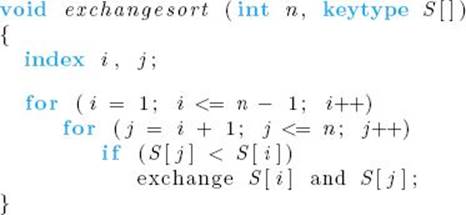
Suppose that currently the array S contains the permutation [2, 4, 3, 1] and we are comparing 2 with 1. After that comparison, 2 and 1 will be exchanged, thereby removing the inversions (2, 1), (4, 1), and (3, 1). However, the inversions (4, 2) and (3, 2) have been added, and the net reduction in inversions is only one. This example illustrates the general result that Exchange Sort always has a net reduction of at most one inversion after each comparison.
Because Insertion Sort’s worst-case time complexity is n (n − 1) /2 and its average-case time complexity is about n2/4, it is about as good as we can hope to do (as far as comparisons of keys are concerned) with algorithms that sort only by comparisons of keys and remove at most one inversion after each comparison. Recall that Mergesort (Algorithms 2.2 and 2.4) and Quicksort (Algorithm 2.6) have time complexities that are better than this. Let’s reinvestigate these algorithms to see how they differ from ones such as Insertion Sort.
7.4 Mergesort Revisited
Mergesort was introduced in Section 2.2. Here we show that it sometimes removes more than one inversion after a comparison. Then, we show how it can be improved.
As mentioned in the proof of Theorem 7.1, algorithms that remove at most one inversion after each comparison will do at least n (n − 1) /2 comparisons when the input is in reverse order. Figure 7.2 illustrates how Mergesort 2 (Algorithm 2.4) handles such an input. When the subarrays [3 4] [1 2] are merged, the comparisons remove more than one inversion. After 3 and 1 are compared, 1 is put in the first array slot, thereby removing the inversions (3, 1) and (4, 1).
Figure 7.2 Mergesort sorting an input that is in reverse order.
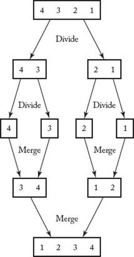
After 3 and 2 are compared, 2 is put in the second array slot, thereby removing the inversions (3, 2) and (4, 2).
Recall that the worst-case time complexity of Mergesort’s number of comparisons of keys is given by
![]()
when n is a power of 2, and in general, it is in Θ (n lg n).
We have gained significantly by developing a sorting algorithm that sometimes removes more than one inversion after a comparison. Recall from Section 1.4.1 that Θ (n lg n) algorithms can handle very large inputs, whereas quadratic-time algorithms cannot.
Using the method of “generating functions” for solving recurrence, we can show that the average-case time complexity of Mergesort’s number of comparison of keys, when n is a power of 2, is given by
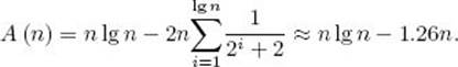
Although that method is not discussed in Appendix B, it can be found in Sahni (1988). The average case is not much better than the worst case.
It is left as an exercise to show that the every-case time complexity of the number of assignments of records done by Mergesort is given approximately by
![]()
Next we analyze the space usage for Mergesort.
Analysis of Algorithm 7.2
![]() Analysis of Extra Space Usage (Mergesort 2)
Analysis of Extra Space Usage (Mergesort 2)
As discussed in Section 2.2, even the improved version of Mergesort given in Algorithm 2.4 requires an entire additional array of size n. Furthermore, while the algorithm is sorting the first subarray, the values of mid, mid+1, low, and high need to be stored in the stack of activation records. Because the array is always split in the middle, this stack grows to a depth of ![]() lg n
lg n![]() . The space for the additional array of records dominates, which means that in every case the extra space usage is in Θ (n) records. By “in Θ (n) records” we mean that the number of records is in Θ (n).
. The space for the additional array of records dominates, which means that in every case the extra space usage is in Θ (n) records. By “in Θ (n) records” we mean that the number of records is in Θ (n).
Improvements of Mergesort
We can improve the basic Mergesort algorithm in three ways. One is a dynamic programming version of Mergesort, another is a linked version, and the third is a more complex merge algorithm.
For the first improvement, look again at the example of applying Mergesort in Figure 2.2. If you were going to do a mergesort by hand, you would not need to divide the array until singletons were reached. Rather you could simply start with singletons, merge the singletons into groups of two, then into groups of four, and so on until the array was sorted. We can write an iterative version of Mergesort that mimics this method, and we can thereby avoid the overhead of the stack operations needed to implement recursion. Notice that this is a dynamic programming approach to Mergesort. The algorithm for this version follows. The loop in the algorithm treats the array size as a power of 2. Values of n that are not powers of 2 are handled by going through the loop 2![]() lg n
lg n![]() times but simply not merging beyond n.
times but simply not merging beyond n.
![]() Algorithm 7.3
Algorithm 7.3
Mergesort 3 (Dynamic Programming Version)
Problem: Sort n keys in nondecreasing order.
Inputs: positive integer n; array of keys S indexed from 1 to n.
Outputs: the array S containing the keys in nondecreasing order.
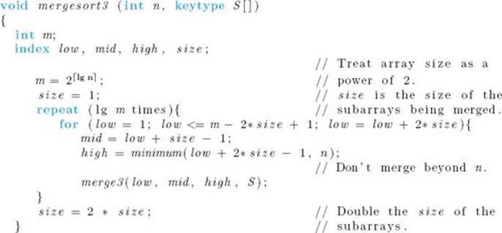
With this improvement, we can also decrease the number of assignments of records. The array U, which is defined locally in procedure merge2 (Algorithm 2.5), can be defined locally in mergesort3 as an array indexed from 1 to n. After the first pass through the repeat loop, U will contain theitems in S with pairs of singletons merged. There is no need to copy these items back to S, as is done at the end of merge2 . Instead, in the next pass through the repeat loop, we can simply merge the items in U into S. That is, we reverse the roles of the two arrays. In each subsequent pass we keep reversing the roles. It is left as an exercise to write versions of mergesort3 and merge3 that do this. In this way we reduce the number of assignments of records from about 2n lg n to about n lg n. We have established that the every-case time complexity of the number of assignments of records done by Algorithm 7.3 is given approximately by
![]()
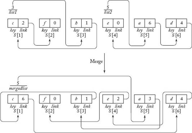
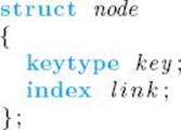
The second improvement of Mergesort is a linked version of the algorithm. As discussed in Section 7.1, the Sorting problem ordinarily involves sorting of records according to the values of their keys. If the records are large, the amount of extra space used by Mergesort can be considerable. We can reduce the extra space by adding a link field to each record. We then sort the records into a sorted linked list by adjusting the links rather than by moving the records. This means that an extra array of records need not be created. Because the space occupied by a link is considerably less than that of a large record, the amount of space saved is significant. Furthermore, there will be a time savings because the time required to adjust links is less than that needed to move large records. Figure 7.3 illustrates how the merging is accomplished using links. The algorithm that follows contains this modification. We present Mergesort and Merge as one algorithm because we need not analyze them further. Mergesort is written recursively for the sake of readability. Of course, the iterative improvement mentioned previously can be implemented along with this improvement. If we used both iteration and links, the improvement of repeatedly reversing the roles of U and S would not be included because no extra array is needed when linked lists are merged. The data type for the items in the array S in this algorithm is as follows:
Figure 7.3 Merging using links. Arrows are used to show how the links work. The keys are letters to avoid confusion with indices.
![]() Algorithm 7.4
Algorithm 7.4
Mergesort 4 (Linked Version)
Problem: Sort n keys in nondecreasing order.
Inputs: positive integer n; array of records, S, of the type just given, indexed from 1 to n.
Outputs: the array S with the values in the key field sorted in nondecreasing order. The records are in an ordered linked list using the link field.
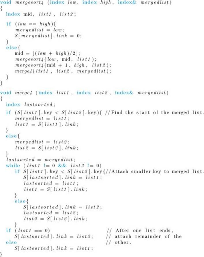
It is not necessary to check whether list1 or list2 is 0 on entry to merge4 because mergesort4 never passes an empty list to merge4 . As was the case for Algorithm 2.4 (Mergesort 2), n and S are not inputs to mergesort4 . The top level call would be
mergesort4 (1, n, listfront);
After execution, listfront would contain the index of the first record in the sorted list.
After sorting, we often want the records to be in sorted sequence in contiguous array slots (that is, sorted in the usual way) so that we can access them quickly by the key field using Binary Search (Algorithm 2.1). Once the records have been sorted according to the links, it is possible to rearrange them so that they are in sorted sequence in contiguous array slots using an in-place, Θ (n) algorithm. In the exercises you are asked to write such an algorithm.
This improvement of Mergesort accomplishes two things. First, it replaces the need for n additional records with the need for only n links. That is, we have the following:
Analysis of Algorithm 7.4
![]() Analysis of Extra Space Usage (Mergesort 4)
Analysis of Extra Space Usage (Mergesort 4)
In every case, the extra space usage is in Θ (n) links. By “in Θ (n) links” we mean that the number of links is in Θ (n).
Second, it reduces the time complexity of the number of assignments of records to 0 if we do not need to have the records ordered in contiguous array slots and to Θ (n) if we do.
The third improvement of Mergesort is a more complex merge algorithm that is presented in Huang and Langston (1988). That merge algorithm is also Θ (n) but with a smalI, constant amount of additional space.
7.5 Quicksort Revisited
As a refresher, let’s first repeat the algorithm for Quicksort:
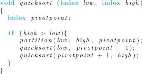
Although its worst-case time complexity is quadratic, we saw in Section 2.4 that the average-case time complexity of Quicksort’s number of comparisons of keys is given by
![]()
which is not much worse than Mergesort. Quicksort has the advantage over Mergesort in that no extra array is needed. However, it is still not an in-place sort because, while the algorithm is sorting the first subarray, the first and last indices of the other subarray need to be stored in the stack of activation records. Unlike Mergesort, we have no guarantee that the array will always be split in the middle. In the worse case, partition may repeatedly split the array into an empty subarray on the right and a subarray with one less item on the left. In this way, n − 1 pairs of indices will end up being stacked, which means that the worst-case extra space usage is in Θ(n). It is possible to modify Quicksort so that the extra space usage is at most about lg n. Before showing this and other improvements of Quicksort, let’s discuss the time complexity of the number of assignments of records by Quicksort.
In the exercises, you are asked to establish that the average number of exchanges performed by Quicksort is about 0.69 (n + 1) lg n. Assuming that three assignments are done to perform one exchange, the average-case time complexity of the number of assignments of records done by Quicksortis given by
![]()
Improvements of the Basic Quicksort Algorithm
We can reduce the extra space usage of Quicksort in five different ways. First, in procedure quicksort, we determine which subarray is larger and always stack that one while the other is sorted. The following is an analysis of the space used by this version of quicksort.
![]() Analysis of Extra Space Usage (Improved Quicksort)
Analysis of Extra Space Usage (Improved Quicksort)
In this version, the worst-case space usage occurs when partition splits the array exactly in half each time, resulting in a stack depth about equal to lg n. Therefore, the worst-case space usage is in Θ (lg n) indices.
Second, as discussed in the exercises, there is a version of partition that cuts the average number of assignments of records significantly. For that version, the average-case time complexity of the number of assignments of records done by Quicksort is given by
![]()
Third, each of the recursive calls in procedure quicksort causes low, high, and pivotpoint to be stacked. A good deal of the pushing and popping is unnecessary. While the first recursive call to quicksort is being processed, only the values of pivotpoint and high need to be saved on the stack. While the second recursive call is being processed, nothing needs to be saved. We can avoid the unnecessary operations by writing quicksort iteratively and manipulating the stack in the procedure. That is, we do explicit stacking instead of stacking by recursion. You are asked to do this in the exercises.
Fourth, as discussed in Section 2.7, recursive algorithms such as Quicksort can be improved by determining a threshold value at which the algorithm calls an iterative algorithm instead of dividing an instance further.
Finally, as mentioned in the worst-case analysis of Algorithm 2.6 (Quicksort), the algorithm is least efficient when the input array is already sorted. The closer the input array is to being sorted, the closer we are to this worst-case performance. Therefore, if there is reason to believe that the array may be close to already being sorted, we can improve the performance by not always choosing the first item as the pivot item. One good strategy to use in this case is to choose the median of S [low], S[![]() L (low + high) /2
L (low + high) /2![]() ], and S [high] for the pivot point. Of course, if we have no reason to believe that there is any particular structure in the input array, choosing any item for the pivot item is, on the average, just as good as choosing any other item. In this case, all we really gain by taking the median is the guarantee that one of the subarrays will not be empty (as long as the three values are distinct).
], and S [high] for the pivot point. Of course, if we have no reason to believe that there is any particular structure in the input array, choosing any item for the pivot item is, on the average, just as good as choosing any other item. In this case, all we really gain by taking the median is the guarantee that one of the subarrays will not be empty (as long as the three values are distinct).
7.6 Heapsort
Unlike Mergesort and Quicksort, Heapsort is an in-place Θ (n lg n) algorithm. First we review heaps and describe basic heap routines needed for sorting using heaps. Then we show how to implement these routines.
• 7.6.1 Heaps and Basic Heap Routines
Recall that the depth of a node in a tree is the number of edges in the unique path from the root to that node, the depth d of a tree is the maximum depth of all nodes in the tree, and a leaf in a tree is any node with no children (see Section 3.5). An internal node in a tree is any node that has at least one child. That is, it is any node that is not a leaf. A complete binary tree is a binary tree that satisfies the following conditions:
• All internal nodes have two children.
• All leaves have depth d.
An essentially complete binary tree is a binary tree that satisfies the following conditions:
• It is a complete binary tree down to a depth of d − 1.
• The nodes with depth d are as far to the left as possible.
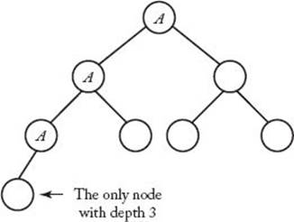
Although essentially complete binary trees are difficult to define, it is straightforward to grasp their properties from a picture. Figure 7.4 shows an essentially complete binary tree.
We can now define a heap. A heap is an essentially complete binary tree such that
Figure 7.4 An essentially complete binary tree.
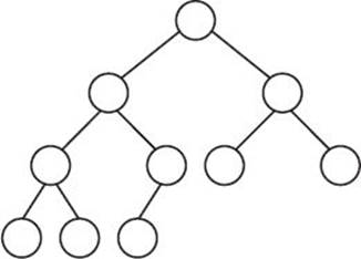
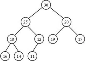
Figure 7.5 A heap.
• The values stored at the nodes come from an ordered set.
• The value stored at each node is greater than or equal to the values stored at its children. This is called the heap property.
Figure 7.5 shows a heap. Because we are presently interested in sorting, we will refer to the items stored in the heap as keys.
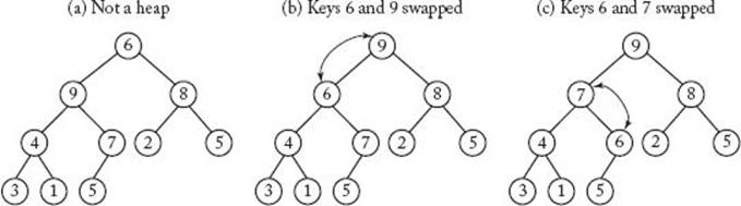
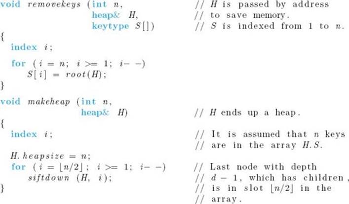
Suppose that somehow we have arranged the keys that are to be sorted in a heap. If we repeatedly remove the key stored at the root while maintaining the heap property, the keys will be removed in nonincreasing sequence. If, while removing them, we place them in an array starting with the nth slot and going down to the first slot, they will be sorted in nondecreasing sequence in the array. After removing the key at the root, we can restore the heap property by replacing the key at the root with the key stored at the bottom node (by “bottom node” we mean the far-right leaf), deleting the bottom node, and calling a procedure siftdown that “sifts” the key now at the root down the heap until the heap property is restored. The sifting is accomplished by initially comparing the key at the root with the larger of the keys at the children of the root. If the key at the root is smaller, the keys are exchanged. This process is repeated down the tree until the key at a node is not smaller than the larger of the keys at its children. Figure 7.6 illustrates this procedure. High-level pseudocode for it is as follows:
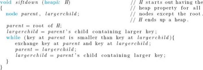
Figure 7.6 Procedure siftdown sifts 6 down until the heap property is restored.
High-level pseudocode for a function that removes the key at the root and restores the heap property is as follows:
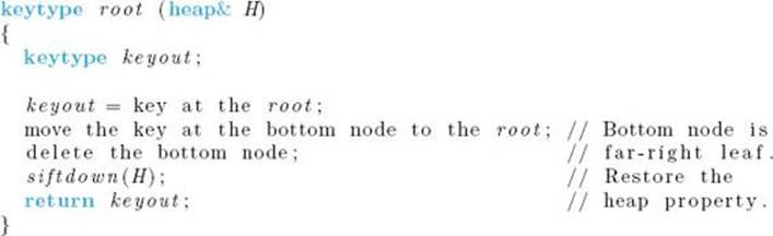
Given a heap of n keys, the following is high-level pseudocode for a procedure that places the keys in sorted sequence into an array S.
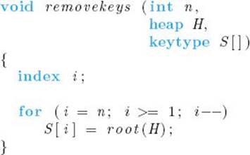
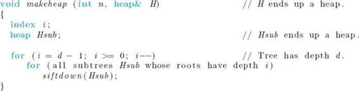
The only task remaining is to arrange the keys in a heap in the first place. Let’s assume that they have been arranged in an essentially complete binary tree that does not necessarily have the heap property (we will see how to do this in the next subsection). We can transform the tree into a heap by repeatedly calling siftdown to perform the following operations: First, transform all subtrees whose roots have depth d−1 into heaps; second, transform all subtrees whose roots have depth d − 2 into heaps; … finally, transform the entire tree (the only subtree whose root has depth 0) into a heap.
Figure 7.7 Using siftdown to make a heap from an essentially complete binary tree. After the steps shown, the right subtree, whose root has depth d – 2, must be made into a heap, and finally the entire tree must be made into a heap.
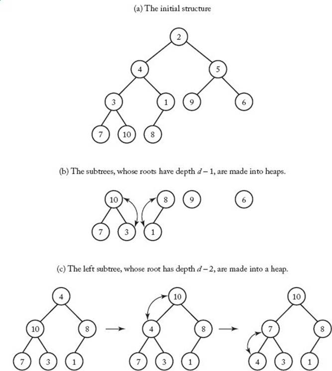
This process is illustrated in Figure 7.7 and is implemented by the procedure outlined in the following high-level pseudocode.
Finally, we present high-level pseudocode for Heapsort (it is assumed that the keys are already arranged in an essentially complete binary tree in H):
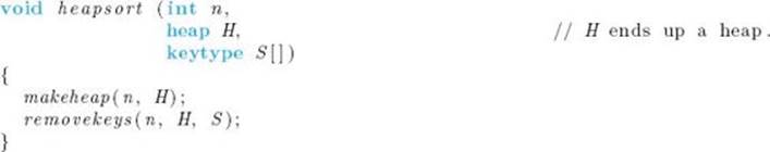
It may seem that we were not telling the truth earlier because this Heapsort algorithm does not appear to be an in-place sort. That is, we need extra space for the heap. However, next we implement a heap using an array. We show that the same array that stores the input (the keys to be sorted) can be used to implement the heap, and that we never simultaneously need the same array slot for more than one purpose.
• 7.6.2 An Implementation of Heapsort
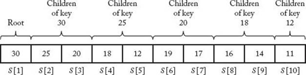
We can represent an essentialIy complete binary tree in an array by storing the root in the first array slot, the root’s left and right children in the second and third slots, respectively, the left and right children of the root’s left child in the fourth and fifth array slots, and so on. The array representation of the heap in Figure 7.5 is shown in Figure 7.8. Notice that the index of the left child of a node is twice that of the node, and the index of the right child is 1 greater than twice that of the node. Recall that in the high-level pseudocode for Heapsort, we required that the keys initially be in an essentially complete binary tree. If we place the keys in an array in an arbitrary order, they will be structured in some essentially complete binary tree according to the representation just discussed. The following low-level pseudocode uses that representation.
Figure 7.8 The array representation of the heap in Figure 7.5.
![]() Heap Data Structure
Heap Data Structure
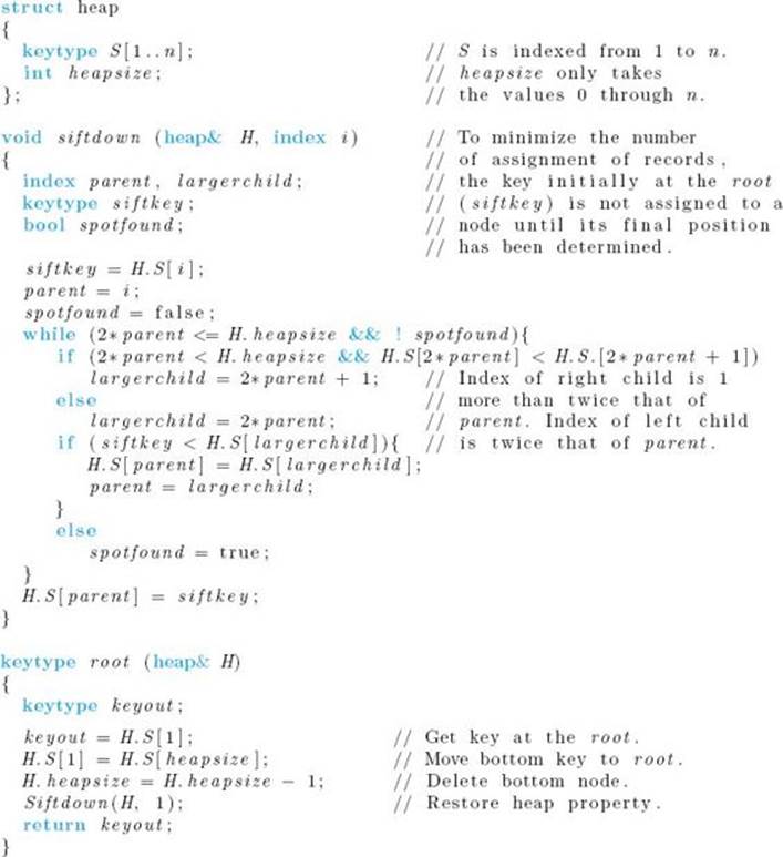
We can now give an algorithm for Heapsort. The algorithm assumes that the keys to be sorted are already in H.S. This automatically structures them in an essentially complete binary tree according to the representation in Figure 7.8. After the essentially complete binary tree is made into a heap, the keys are deleted from the heap starting with the nth array slot and going down to the first array slot. Because they are placed in sorted sequence in the output array in that same order, we can use H.S as the output array with no possibility of overwriting a key in the heap. This strategy gives us the in-place algorithm that follows.
![]() Algorithm 7.5
Algorithm 7.5
Heapsort
Problem: Sort n keys in nondecreasing order.
Inputs: positive integer n, array of n keys stored in an array implementation H of a heap.
Outputs: the keys in nondecreasing order in the array H.S.
Analysis of Algorithm 7.5
![]() Worst-Case Time CompIexity Analysis of Number of Comparisons of Keys (Heapsort)
Worst-Case Time CompIexity Analysis of Number of Comparisons of Keys (Heapsort)
Basic instruction: the comparisons of keys in procedure siftdown.
Input size: n, the number of keys to be sorted.
Procedures makeheap and removekeys both call siftdown. We analyze these procedures separately. We do the analysis for n a power of 2 and then use Theorem B.4 in Appendix B to extend the result to n in general.
Analysis of makeheap
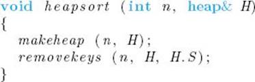
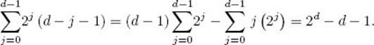
Let d be the depth of the essentially complete binary tree that is the input. Figure 7.9 illustrates that when n is a power of 2, the depth d of the tree is lg n, there is exactly one node with that depth, and that node has d ancestors. When the heap is constructed, all the keys in ancestors of the node with level d will possibly be sifted through one more node (that is, the node with level d) than they would be sifted through if that node were not there. All other keys would be sifted through the same number of nodes as they would be if that node were not there. We first obtain an upper bound on the total number of nodes through which all keys would be sifted if the node with depth d were not there. Because that node has d ancestors and the key at each of these ancestors will possibly be sifted through one more node, we can add d to this upper bound to obtain our actual upper bound on the total number of nodes through which all keys are sifted. To that end, if the node with depth d were not there, each key initially at a node with depth d − 1 would be sifted through 0 nodes when the heap was constructed; each key initially at a node with depth d − 2 would be sifted through at most one node; and so on until finally the key at the root would be sifted through at most d−1 nodes. It is left as an exercise to show that, when n is a power of 2, there are 2j nodes with depth j for 0 ≤ j < d. For n a power of 2, the following table shows the number of nodes with each depth and at most the number of nodes through which a key at that depth would be sifted (if the node with depth d were not there):
Figure 7.9 An illustration using n = 8, showing that if an essentially complete binary tree has n nodes and n is a power of 2, then the depth d of the tree is lg n, there is one node with depth d, and that node has d ancestors. The three ancestors of that node are marked “A.”
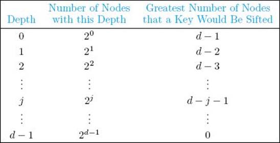
Therefore, the number of nodes through which all keys would be sifted, if the node with depth d were not there, is at most
The last equality is obtained by applying results in Examples A.3 and A.5 in Appendix A and doing some algebraic manipulations. Recall that we need to add d to this bound to obtain the actual upper bound on the total number of nodes through which all keys are sifted. Therefore, the actual upper bound is
![]()
The second equality is a result of the fact that d = lg n when n is a power of 2. Each time a key is sifted through one node, there is one pass through the while loop in procedure siftdown. Because there are two comparisons of keys in each pass through that loop, the number of comparisons of keys done by makeheap is at most
![]()
It is a somewhat surprising result that the heap can be constructed in linear time. If we could remove the keys in linear time, we would have a linear-time sorting algorithm. As we shall see, however, this is not the case.
Analysis of removekeys
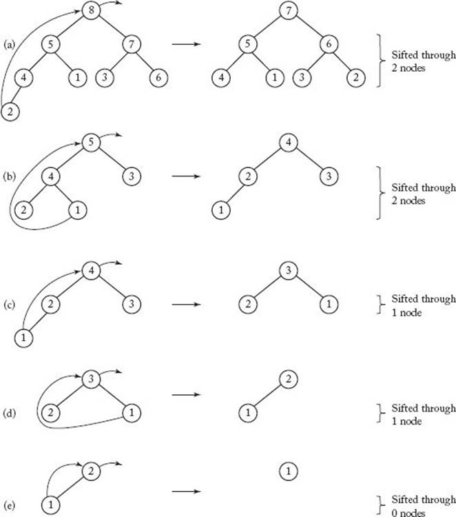
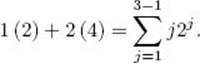
Figure 7.10 illustrates the case in which n = 8 and d = lg 8 = 3. As shown in Figure 7.10(a) and (b), when the first and fourth keys are each removed, the key moved to the root sifts through at most d − 1 = 2 nodes. Clearly, the same thing happens for the two keys between the first and the fourth. Therefore, when the first four keys are removed, the key moved to the root sifts through at most two nodes. As shown in Figure 7.10(c) and (d), when each of the next two keys is removed, the key moved to the root sifts through at most d − 2 = 1 node. Finally, Figure 7.10(e) shows that, when the next key is removed, the key moved to the root sifts through 0 nodes. Clearly, there is also no sifting when the last key is removed. The total number of nodes through which all keys are sifted is at most
Figure 7.10 Removing the keys from a heap with eight nodes. The removal of the first key is depicted in (a); the fourth in (b); the fifth in (c); the sixth in (d); and the seventh in (e). The key moved to the root is sifted through the number of nodes shown on the right.
It is not hard to see that this result can be extended to n an arbitrary power of 2. Because each time a key is sifted through one node, there is one pass through the while loop in procedure siftdown, and, because there are two comparisons of keys in each pass through that loop, the number of comparisons of keys done by removekeys is at most
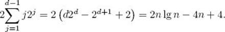
The first equality is obtained by applying the result in Example A.5 in Appendix A and doing some algebraic manipulations, whereas the second results from the fact that d = lg n when n is a power of 2.
Combining the Two Analyses
The combined analyses of makeheap and removekeys show that the number of comparisons of keys in heapsort is at most
![]()
when n is a power of 2. Showing that there is a case in which we have this number of comparisons is left as an exercise. Therefore, for n a power of 2,
![]()
It is possible to show that W (n) is eventually nondecreasing. Therefore, Theorem B.4 in Appendix B implies that, for n in general,
![]()
It appears to be difficult to analyze Heapsort’s average-case time complexity analytically. However, empirical studies have shown that its average case is not much better than its worse case. This means that the average-case time complexity of the number of comparisons of keys done by Heapsortis approximated by
![]()
In the exercises, you are asked to establish that the worst-case time complexity of the number of assignments of records done by Heapsort is approximated by
![]()
As is the case for the comparisons of keys, Heapsort does not do much better than this on the average.
Finally, as already discussed, we have the following space usage.
Analysis of Algorithm 7.5
![]() Analysis of Extra Space Usage (Heapsort)
Analysis of Extra Space Usage (Heapsort)
Heapsort is an in-place sort, which means that the extra space is in Θ (1).
As mentioned in Section 7.2, Heapsort is an example of a selection sort because it sorts by selecting records in order and placing them in their proper sorted positions. It is the call to removekeys that places a record in its proper sorted position.
7.7 Comparison of Mergesort, Quicksort, and Heapsort
Table 7.2 summarizes our results concerning the three algorithms. Because Heapsort is, on the average, worse than Quicksort in terms of both comparisons of keys and assignments of records, and because Quicksort’s extra space usage is minimal, Quicksort is usually preferred to Heapsort. Because our original implementation of Mergesort (Algorithms 2.2 and 2.4) uses an entire additional array of records, and because Mergesort always does about three times as many assignments of records as Quicksort does on the average, Quicksort is usually preferred to Mergesort even though Quicksort does slightly more comparisons of keys on the average. However, the linked implementation of Mergesort (Algorithm 7.4) eliminates almost all the disadvantages of Mergesort. The only disadvantage remaining is the additional space used for Θ (n) extra links.
• Table 7.2 Analysis summary for Θ (n lg n) sorting algorithms*
*Entries are approximate; the average cases for Mergesort and Heapsort are slightly better than the worst cases.
†If it is required that the records be in sorted sequence in contiguous array slots, the worst case is in Θ (n).
7.8 Lower Bounds for Sorting Only by Comparison of Keys
We have developed Θ (n lg n) sorting algorithms, which represent a substantial improvement over quadratic-time algorithms. A good question is whether we can develop sorting algorithms whose time complexities are of even better order. We show that, as long as we limit ourselves to sorting only by comparisons of keys, such algorithms are not possible.
Although our results still hold if we consider probabilistic sorting algorithms, we obtain the results for deterministic sorting algorithms. (See Section 5.3 for a discussion of probabilistic and deterministic algorithms.) As done in Section 7.3, we obtain our results under the assumption that the nkeys are distinct. Furthermore, as discussed in that section, we can assume that the n keys are simply the positive integers 1, 2, … , n, because we can substitute 1 for the smallest key, 2 for the second smallest, and so on.
• 7.8.1 Decision Trees for Sorting Algorithms
Consider the following algorithm for sorting three keys.
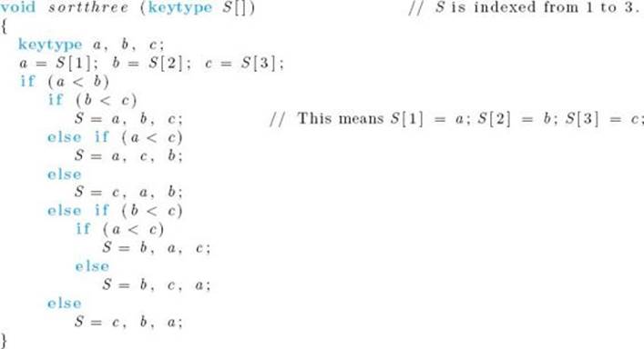
We can associate a binary tree with procedure sortthree as follows. We place the comparison of a and b at the root. The left child of the root contains the comparison that is made if a < b, whereas the right child contains the comparison that is made if a ≥ b. We proceed downward, creating nodes in the tree until all possible comparisons done by the algorithm are assigned nodes. The sorted keys are stored at the leaves. Figure 7.11 shows the entire tree. This tree is called a decision tree because at each node a decision must be made as to which node to visit next. The action of proceduresortthree on a particular input corresponds to following the unique path from the root to a leaf, determined by that input. There is a leaf in the tree for every permutation of three keys, because the algorithm can sort every possible input of size 3.
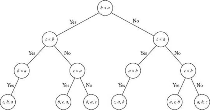
A decision tree is called valid for sorting n keys if, for each permutation of the n keys, there is a path from the root to a leaf that sorts that permutation. That is, it can sort every input of size n. For example, the decision tree in Figure 7.11 is valid for sorting three keys, but would no longer be valid if we removed any branch from the tree. To every deterministic algorithm for sorting n keys, there corresponds at least one valid decision tree. The decision tree in Figure 7.11 corresponds to procedure sortthree, and the decision tree in Figure 7.12 corresponds to Exchange Sort when sorting three keys. (You are encouraged to verify this.) In that tree, a, b, and c are again the initial values of S [1], S [2], and S [3]. When a node contains, for example, the comparison “c < b,” this does not mean that Exchange Sort compares S [3] with S [2] at that point; rather, it means that Exchange Sort compares the array item whose current value is c with the one whose current value is b. In the tree in Figure 7.12, notice that the level-2 node containing the comparison “b < a” has no right child. The reason is that a “no” answer to that comparison contradicts the answers obtained on the path leading to that node, which means that its right child could not be reached by making a consistent sequence of decisions starting at the root. Exchange Sort makes an unnecessary comparison at this point, because Exchange Sort does not “know” that the answer to the question must be “yes.” This often happens in suboptimal sorting algorithms. We say that a decision tree is pruned if every leaf can be reached from the root by making a consistent sequence of decisions. The decision tree in Figure 7.12 is pruned, whereas it would not be pruned if we added a right child to the node just discussed, even though it would still be valid and would still correspond to Exchange Sort. Clearly, to every deterministic algorithm for sorting n keys there corresponds a pruned, valid decision tree. Therefore, we have the following lemma.
Figure 7.11 The decision tree corresponding to procedure sortthree.
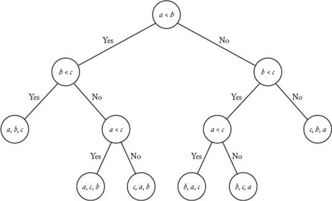
Figure 7.12 The decision tree corresponding to Exchange Sort when sorting three keys.
![]() Lemma 7.1
Lemma 7.1
To every deterministic algorithm for sorting n distinct keys there corresponds a pruned, valid, binary decision tree containing exactly n! leaves.
Proof: As just mentioned, there is a pruned, valid decision tree corresponding to any algorithm for sorting n keys. When all the keys are distinct, the result of a comparison is always “<” or “>.” Therefore, each node in that tree has at most two children, which means that it is a binary tree. Next we show that it has n! leaves. Because there are n! different inputs that contain n distinct keys and because a decision tree is valid for sorting n distinct keys only if it has a leaf for every input, the tree has at least n! leaves. Because there is a unique path in the tree for each of the n! different inputs andbecause every leaf in a pruned decision tree must be reachable, the tree can have no more than n! leaves. Therefore, the tree has exactly n! leaves.
Using Lemma 7.1, we can determine bounds for sorting n distinct keys by investigating binary trees with n! leaves. We do this next.
• 7.8.2 Lower Bounds for Worst-Case Behavior
To obtain a bound for the worst-case number of comparisons of keys, we need the following lemma.
![]() Lemma 7.2
Lemma 7.2
The worst-case number of comparisons done by a decision tree is equal to its depth.
Proof: Given some input, the number of comparisons done by a decision tree is the number of internal nodes on the path followed for that input. The number of internal nodes is the same as the length of the path. Therefore, the worst-case number of comparisons done by a decision tree is the length of the longest path to a leaf, which is the depth of the decision tree.
By Lemmas 7.1 and 7.2, we need only find a lower bound on the depth of a binary tree containing n! leaves to obtain our lower bound for the worst-case behavior. The required lower bound on depth is found by means of the following lemmas and theorems.
![]() Lemma 7.3
Lemma 7.3
Proof: We show first that
![]()
Clearly, if a binary tree is not complete, we can create a new binary tree from the original tree by adding leaves such that the new tree has more leaves than the original tree and has the same depth as the original tree. Therefore it suffices to obtain Equality 7.1 for complete binary trees. Actually, for complete binary trees, we will obtain equality. The proof is by induction.
Induction base: The (complete) binary tree with depth 0 has one node that is both the root and the only leaf. Therefore, for this tree, the number of
leaves m equals 1, and
![]()
Induction hypothesis: Assume that for the complete binary tree with depth d,
![]()
where m is the number of leaves.
Induction step: We need to show that, for the complete binary tree with depth d + 1,
![]()
where m’ is the number of leaves. We can obtain the complete binary tree with depth d + 1 from the complete binary tree with depth d by giving each leaf in this latter tree exactly two children, which are then the only leaves in the new tree. Therefore,
![]()
Owing to this equality and the induction hypothesis, we have
![]()
which completes the induction proof.
Taking the lg of both sides of Inequality 7.1 yields
![]()
Because d is an integer, this implies
![]()
![]() Theorem 7.2
Theorem 7.2
Any deterministic algorithm that sorts n distinct keys only by comparisons of keys must in the worst case do at least
![]()
Proof: By Lemma 7.1, to any such algorithm there corresponds a pruned, valid, binary decision tree containing n! leaves. By Lemma 7.3, the depth of that tree is greater than or equal to ![]() lg (n!)
lg (n!)![]() . The theorem now follows, because Lemma 7.2 says that any decision tree’s worst-case number of comparisons is given by its depth.
. The theorem now follows, because Lemma 7.2 says that any decision tree’s worst-case number of comparisons is given by its depth.
How does this bound compare with the worst-case performance of Mergesort—namely, n lg n − (n − 1)? Lemma 7.4 enables us to compare the two.
![]() Lemma 7.4
Lemma 7.4
For any positive integer n,
![]()
Proof: The proof requires knowledge of integral calculus. We have
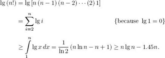
![]() Theorem 7.3
Theorem 7.3
Any deterministic algorithm that sorts n distinct keys only by comparisons of keys must in the worst case do at least
![]()
Proof: The proof follows from Theorem 7.2 and Lemma 7.4.
We see that Mergesort’s worst-case performance of n lg n − (n − 1) is close to optimal. Next we show that this also holds for its average-case performance.
• 7.8.3 Lower Bounds for Average-Case Behavior
We obtain our results under the assumption that all possible permutations are equally likely to be the input.
If the pruned, valid, binary decision tree corresponding to a deterministic sorting algorithm for sorting n distinct keys contains any comparison nodes with only one child (as is the case for the tree in Figure 7.12), we can replace each such node by its child and prune the child to obtain a decision tree that sorts using no more comparisons than did the original tree. Every nonleaf in the new tree will contain exactly two children. A binary tree in which every nonleaf contains exactly two children is called a 2-tree. We summarize this result with the following lemma.
![]() Lemma 7.5
Lemma 7.5
To every pruned, valid, binary decision tree for sorting n distinct keys, there corresponds a pruned, valid decision 2-tree that is at least as efficient as the original tree.
Proof: The proof follows from the preceding discussion.
The external path length (EPL) of a tree is the total length of all paths from the root to the leaves. For example, for the tree in Figure 7.11,
![]()
Recall that the number of comparisons done by a decision tree to reach a leaf is the length of the path to the leaf. Therefore, the EPL of a decision tree is the total number of comparisons done by the decision tree to sort all possible inputs. Because there are n! different inputs of size n (when all keys are distinct) and because we are assuming all inputs to be equally likely, the average number of comparisons done by a decision tree for sorting n distinct keys is given by
![]()
This result enables us to prove an important lemma. First we define minEPL(m) as the minimum of the EPL of 2-trees containing m leaves. The lemma now follows.
![]() Lemma 7.6
Lemma 7.6
Any deterministic algorithm that sorts n distinct keys only by comparisons of keys must on the average do at least
![]()
Proof: Lemma 7.1 says that to every deterministic algorithm for sorting n distinct keys there corresponds a pruned, valid, binary decision tree containing n leaves. Lemma 7.5 says that we can convert that decision tree to a 2-tree that is at least as efficient as the original tree. Because the original tree has n! leaves, so must the 2-tree we obtain from it. The lemma now follows from the preceding discussion.
By Lemma 7.6, to obtain a lower bound for the average case, we need only find a lower bound for minEPL(m), which is accomplished by means of the following four lemmas.
![]() Lemma 7.7
Lemma 7.7
Any 2-tree that has m leaves and whose EPL equals minEPL(m) must have all of its leaves on at most the bottom two levels.
Proof: Suppose that some 2-tree does not have all of its leaves on the bottom two levels. Let d be the depth of the tree, let A be a leaf in the tree that is not on one of the bottom two levels, and let k be the depth of A. Because nodes at the bottom level have depth d,
![]()
We show that this tree cannot minimize the EPL among trees with the same number of leaves, by developing a 2-tree with the same number of leaves and a lower EPL. We can do this by choosing a nonleaf B at level d − 1 in our original tree, removing its two children, and giving two children toA, as illustrated in Figure 7.13. Clearly, the new tree has the same number of leaves as the original tree. In our new tree, neither A nor the children of B are leaves, but they are leaves in our old tree. Therefore, we have decreased the EPL by the length of the path to A and by the lengths of the two paths to B’s children. That is, we have decreased the EPL by
![]()
In our new tree, B and the two new children of A are leaves, but they are not leaves in our old tree. Therefore, we have increased the EPL by the length of the path to B and the lengths of the two paths to A’s new children. That is, we have increased the EPL by
![]()
The net change in the EPL is
![]()
Figure 7.13 The trees in (a) and (b) have the same number of leaves, but the tree in (b) has a smaller EPL.
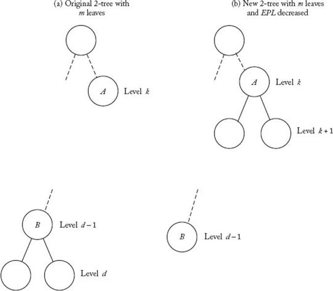
The inequality occurs because k ≤ d − 2. Because the net change in the EPL is negative, the new tree has a smaller EPL. This completes the proof that the old tree cannot minimize the EPL among trees with the same number of leaves.
![]() Lemma 7.8
Lemma 7.8
Any 2-tree that has m leaves and whose EPL equals minEPL(m) must have
![]()
and have no other leaves, where d is the depth of the tree.
Proof: Because Lemma 7.7 says that all leaves are at the bottom two levels and because nonleaves in a 2-tree must have two children, it is not hard to see that there must be 2d − 1 nodes at level d − 1. Therefore, if r is the number of leaves at level d − 1, the number of nonleaves at that level is 2d − 1 − r. Because nonleaves in a 2-tree have exactly two children, for every nonleaf at level d − 1, there are two leaves at level d. Because these are the only leaves at level d, the number of leaves at level d is equal to 2 (2d − 1 − r). Because Lemma 7.7 says that all leaves are at level d or d − 1,
![]()
Simplifying yields
![]()
Therefore, the number of leaves at level d is
![]()
![]() Lemma 7.9
Lemma 7.9
For any 2-tree that has m leaves and whose EPL equals minEPL(m), the depth d is given by
![]()
Proof: We prove the case where m is a power of 2. The proof of the general case is left as an exercise. If m is a power of 2, then, for some integer k,
![]()
Let d be the depth of a minimizing tree. As in Lemma 7.8, let r be the number of leaves at level d − 1. By that lemma,
![]()
Because r ≥ 0, we must have d ≥ k. We show that assuming d > k leads to a contradiction. If d > k, then
![]()
Because r ≤ m, this means that r = m, and all leaves are at level d − 1. But there must be some leaves at level d. This contradiction implies that d = k, which means that r = 0. Because r = 0,
![]()
which means that d = lg m. Because lg m = ![]() lg m
lg m![]() when m is a power of 2, this completes the proof.
when m is a power of 2, this completes the proof.
![]() Lemma 7.10
Lemma 7.10
For all integers m ≥ 1
![]()
Proof: By Lemma 7.8, any 2-tree that minimizes this EPL must have 2d leaves at level d−1, have 2m−2d leaves at level d, and have no other leaves. We therefore have
![]()
Therefore, by Lemma 7.9,
![]()
If m is a power of 2, this expression clearly equals m lg m, which equals m ![]() lg m
lg m![]() , which equals m
, which equals m![]() lg m
lg m![]() in this case. If m is not a power of 2, then
in this case. If m is not a power of 2, then ![]() lg m
lg m![]() =
= ![]() lg m
lg m![]() + 1. So, in this case,
+ 1. So, in this case,
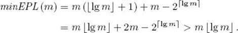
This inequality occurs because, in general, 2m > 2![]() lg m
lg m![]() . This completes the proof.
. This completes the proof.
Now that we have a lower bound for minEPL(m), we can prove our main result.
![]() Theorem 7.4
Theorem 7.4
Any deterministic algorithm that sorts n distinct keys only by comparisons of keys must on the average do at least
![]()
Proof: By Lemma 7.6, any such algorithm must on the average do at least
![]()
By Lemma 7.10, this expression is greater than or equal to
![]()
The proof now follows from Lemma 7.4.
We see that Mergesort’s average-case performance of about n lg n − 1.26n is near optimal for algorithms that sort only by comparisons of keys.
7.9 Sorting by Distribution (Radix Sort)
In the preceding section, we showed that any algorithm that sorts only by comparisons of keys can be no better than Θ (n lg n). If we know nothing about the keys except that they are from an ordered set, we have no choice but to sort by comparing the keys. However, when we have more knowledge we can consider other sorting algorithms. By using additional information about the keys, we next develop one such algorithm.
Suppose we know that the keys are all nonnegative integers represented in base 10. Assuming that they all have the same number of digits, we can first distribute them into distinct piles based on the values of the leftmost digits. That is, keys with the same leftmost digit are placed in the same pile. Each pile can then be distributed into distinct piles based on the values of the second digits from the left. Each new pile can then be distributed into distinct piles based on the values of the third digits from the left, and so on. After we have inspected all the digits, the keys will be sorted. Figure 7.14illustrates this procedure, which is called sorting by distribution, because the keys are distributed into piles.
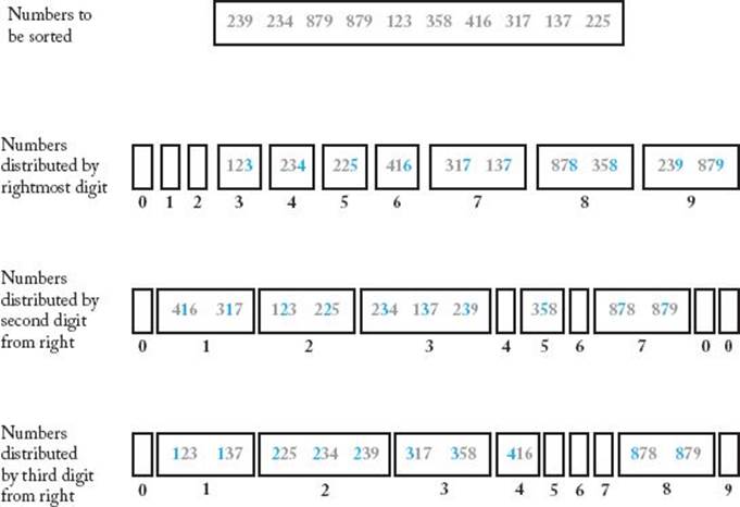
A difficulty with this procedure is that we need a variable number of piles. Suppose instead that we allocate precisely 10 piles (one for each decimal digit), we inspect digits from right to left, and we always place a key in the pile corresponding to the digit currently being inspected. If we do this, the keys still end up sorted as long as we obey the following rule: On each pass, if two keys are to be placed in the same pile, the key coming from the leftmost pile (in the previous pass) is placed to the left of the other key. This procedure is illustrated in Figure 7.15. As an example of how keys are placed, notice that after the first pass, key 416 is in a pile to the left of key 317. Therefore, when they are both placed in the first pile in the second pass, key 416 is placed to the left of key 317. In the third pass, however, key 416 ends up to the right of key 317 because it is placed in the fourth pile, whereas key 317 is placed in the third pile. In this way, the keys end up in the correct order according to their rightmost digits after the first pass, in the correct order according to their two rightmost digits after the second pass, and in the correct order according to all three digits after the third pass, which means they are sorted.
Figure 7.14 Sorting by distribution while inspecting the digits from left to right.
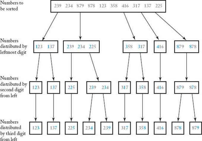
Figure 7.15 Sorting by distribution while inspecting the digits from right to left.
This sorting method precedes computers, having been the method used on the old card-sorting machines. It is called radix sort because the information used to sort the keys is a particular radix (base). The radix could be any number base, or we could use the letters of the alphabet. The number of piles is the same as the radix. For example, if we were sorting numbers represented in hexadecimal, the number of piles would be 16; if we were sorting alpha keys represented in the English alphabet, the number of piles would be 26 because there are 26 letters in that alphabet.
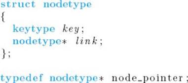
Because the number of keys in a particular pile changes with each pass, a good way to implement the algorithm is to use linked lists. Each pile is represented by a linked list. After each pass, the keys are removed from the lists (piles) by coalescing them into one master linked list. They are ordered in that list according to the lists (piles) from which they were removed. In the next pass, the master list is traversed from the beginning, and each key is placed at the end of the list (pile) to which it belongs in that pass. In this way, the rule just given is obeyed. For readability, we present this algorithm under the assumption that the keys are nonnegative integers represented in base 10. It can be readily modified to sort keys in other radix representations without affecting the order of the time complexity. We need the following declarations for the algorithm.
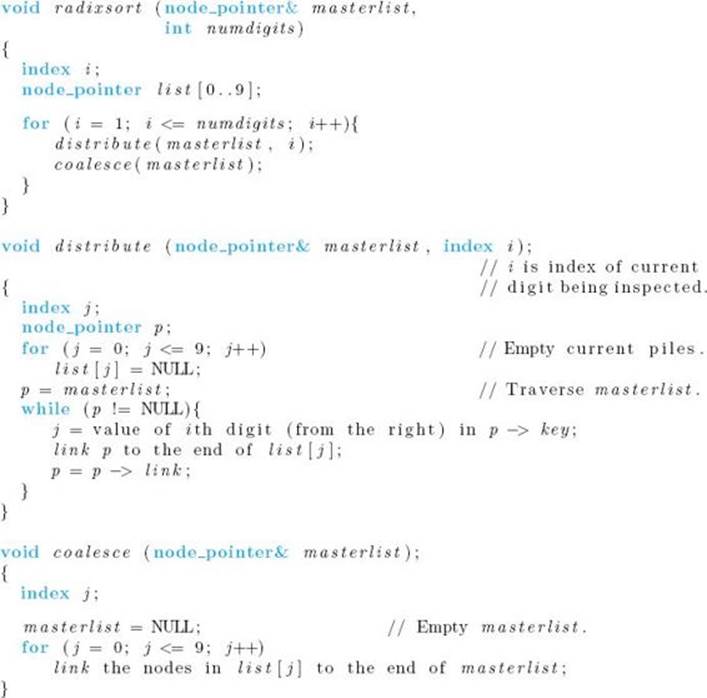
![]() Algorithm 7.6
Algorithm 7.6
Radix Sort
Problem: Sort n nonnegative integers, represented in base 10, in nondecreasing order.
Inputs: linked list masterlist of n nonnegative integers, and an integer numdigits, which is the maximum number of decimal digits in each integer.
Outputs: the linked list masterlist containing the integers in nondecreasing order.
Next we analyze the algorithm.
Analysis of Algorithm 7.6
![]() Every-Case Time Complexity (Radix Sort)
Every-Case Time Complexity (Radix Sort)
Basic operation: Because there are no comparisons of keys in this algorithm, we need to find a different basic operation. In an efficient implementation of coalesce, the lists that contain the piles would have pointers to both their beginnings and their ends so that we can readily add each list to the end of the previous one without traversing the list. Therefore, in each pass through the for loop in that procedure, a list is added to the end of masterlist by simply assigning an address to one pointer variable. We can take that assignment as the basic operation. In procedure distribute, we can take any or all of the instructions in the while loop as the basic operations. Therefore, to have a unit consistent with coalesce, we choose the one that adds a key to the end of a list by assigning an address to a pointer variable.
Input size: n, the number of integers in masterlist, and numdigits, the maximum number of decimal digits in each integer.
Traversal of the entirety of masterlist always requires n passes through the while loop in distribute. Addition of all the lists to masterlist always requires ten passes through the for loop in coalesce. Each of these procedures is called numdigits times from radixsort. Therefore,
![]()
This is not a Θ (n) algorithm because the bound is in terms of numdigits and n. We can create arbitrarily large time complexities in terms of n by making numdigits arbitrarily large. For example, because 1,000,000,000 has 10 digits, it will take Θ (n2) time to sort 10 numbers if the largest one is 1,000,000,000. In practice, the number of digits is ordinarily much smaller than the number of numbers. For example, if we are sorting 1,000,000 social security numbers, n is 1,000,000 whereas numdigits is only 9. It is not hard to see that, when the keys are distinct, the best-case time complexity of Radix Sort is in Θ (n lg n), and ordinarily we achieve the best case.
Next we analyze the extra space used by Radix Sort.
Analysis of Algorithm 7.6
![]() Analysis of Extra Space Usage (Radix Sort)
Analysis of Extra Space Usage (Radix Sort)
No new nodes are ever allocated in the algorithm because a key is never needed simultaneously in masterlist and in a list representing a pile. This means that the only extra space is the space needed to represent the keys in a linked list in the first place. Therefore, the extra space is in Θ (n) links. By “in Θ (n) links” we mean that the number of links is in Θ (n).
EXERCISES
Sections 7.1 and 7.2
1. Implement the Insertion Sort algorithm (Algorithm 7.1), run it on your system, and study its best-case, average-case, and worst-case time complexities using several problem instances.
2. Show that the maximum number of comparisons performed by the Insertion Sort algorithm (Algorithm 7.1) is achieved when the keys are input in nonincreasing order.
3. Show that the worst-case and average-case time complexities for the number of assignments of records performed by the Insertion Sort algorithm (Algorithm 7.1) are given by
![]()
4. Show that the worst-case and average-case time complexities for the number of assignments of records performed by the Exchange Sort algorithm (Algorithm 1.3) are given by
![]()
5. Compare the best-case time complexities of Exchange Sort (Algorithm 1.3) and Insertion Sort (Algorithm 7.1).
6. Is Exchange Sort (Algorithm 1.3) or Insertion Sort (Algorithm 7.1) more appropriate when we need to find in nonincreasing order the k largest (or in nondecreasing order the k smallest) keys in a list of n keys? Justify your answer.
7. Rewrite the Insertion Sort algorithm (Algorithm 7.1) as follows. Include an extra array slot S[0] that has a value smaller than any key. This eliminates the need to compare j with 0 at the top of the while loop. Determine the exact time complexity of this version of the algorithm. Is it better or worse than the time complexity of Algorithm 7.1? Which version should be more efficient? Justify your answer.
8. An algorithm called Shell Sort is inspired by Insertion Sort’s ability to take advantage of the order of the elements in the list. In Shell Sort, the entire list is divided into noncontiguous sublists whose elements are a distance h apart for some number h. Each sublist is then sorted using Insertion Sort. During the next pass, the value of h is reduced, increasing the size of each sublist. Usually the value of each h is chosen to be relatively prime to its previous value. The final pass uses the value 1 for h to sort the list. Write an algorithm for Shell Sort, study its performance, and compare the result with the performance of Insertion Sort.
Section 7.3
9. Show that the permutation [n, n − 1, … , 2, 1] has n (n − 1) inversions.
10. Give the transpose of the permutation [2, 5, 1, 6, 3, 4], and find the number of inversions in both permutations. What is the total number of inversions?
11. Show that there are n (n − 1) /2 inversions in a permutation of n distinct ordered elements with respect to its transpose.
12. Show that the total number of inversions in a permutation and its transpose is n (n − 1) /2. Use this to find the total number of inversions in the permutation in Exercise 10 and its transpose.
Section 7.4 (See also exercises for Section 2.2.)
13. Implement the different Mergesort algorithms discussed in Section 2.2 and Section 7.4, run them on your system, and study their best-case, average-case, and worst-case performances using several problem instances.
14. Show that the time complexity for the number of assignments of records for the Mergesort algorithm (Algorithms 2.2 and 2.4) is approximated by T (n) = 2n lg n.
15. Write an in-place, linear-time algorithm that takes as input the linked list constructed by the Mergesort 4 algorithm (Algorithm 7.4) and stores the records in the contiguous array slots in nondecreasing order according to the values of their keys.
16. Use the divide-and-conquer approach to write a nonrecursive Mergesort algorithm. Analyze your algorithm, and show the results using order notation. Note that it will be necessary to explicitly maintain a stack in your algorithm.
17. Implement the nonrecursive Mergesort algorithm of Exercise 16, run it on your system using the problem instances of Exercise 13, and compare the results to the results of the recursive versions of Mergesort in Exercise 13.
18. Write a version of mergesort3 (Algorithm 7.3), and a corresponding version of merge3, that reverses the rolls of two arrays S and U in each pass through the repeat loop.
Section 7.5 (See also exercises for Section 2.4.)
19. Implement the Quicksort algorithm (Algorithm 2.6) discussed in Section 2.4, run it on your system, and study its best-case, average-case, and worst-case performances using several problem instances.
20. Show that the time complexity for the average number of exchanges performed by the Quicksort algorithm is approximated by 0.69 (n ± 1) lg n.
21. Write a nonrecursive Quicksort algorithm. Analyze your algorithm, and show the results using order notation. Note that it will be necessary to explicitly maintain a stack in your algorithm.
22. Implement the nonrecursive Quicksort algorithm of Exercise 21, run it on your system using the same problem instances you used in Exercise 20, and compare the results to the results of the recursive version of Quicksort in Exercise 20.
23. The following is a faster version of procedure partition, which is called by procedure quicksort.
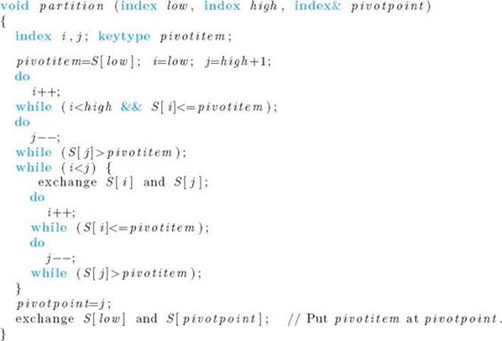
Show that with this partition procedure, the time complexity for the number of assignments of records performed by Quicksort is given by
![]()
Show further that the average-case time complexity for the number of comparisons of keys is about the same as before.
24. Give two instances for which Quicksort algorithm is the most appropriate choice.
25. Another way to sort a list by exchanging out-of-order keys is called Bubble Sort. Bubble Sort scans adjacent pairs of records and exchanges those found to have out-of-order keys. After the first time through the list, the record with the largest key (or the smallest key) is moved to its proper position. This process is done repeatedly on the remaining, unsorted part of the list until the list is completely sorted. Write the Bubble Sort algorithm. Analyze your algorithm, and show the results using order notation. Compare the performance of the Bubble Sort algorithm to those of Insertion Sort, Exchange Sort, and Selection Sort.
Section 7.6
26. Write an algorithm that checks if an essentially complete binary tree is a heap. Analyze your algorithm and show the results using order notation.
27. Show that there are 2j nodes with depth j for j < d in a heap having n (a power of 2) nodes. Here d is the depth of the heap.
28. Show that a heap with n nodes has ![]() n/2
n/2![]() leaves.
leaves.
29. Implement the Heapsort algorithm (Algorithm 7.5), run it on your system, and study its best-case, average-case, and worst-case performances using several problem instances.
30. Show that there is a case for Heapsort in which we get the worst-case time complexity of W (n) ≈ 2n lg n ∈ Θ (n lg n).
31. Show that the worst-case time complexity of the number of assignments of records for Heapsort is approximated by W (n) ≈ n lg n.
32. Modify Heapsort so that it stops after it finds the k largest keys in non-increasing order. Analyze your algorithm, and show the results using order notation.
Section 7.7
33. List all the advantages and disadvantages of all the sorting algorithms discussed in this chapter based on the comparisons of keys and the assignments of records.
34. Run the implementations of all the sorting algorithms discussed in this chapter on your system using several problem instances. Use the results, and the information provided in Exercise 33, to give a detailed comparison of these sorting algorithms.
35. Among Selection Sort, Insertion Sort, Mergesort, Quicksort, and Heapsort, which algorithm would you choose in each list-sorting situation below? Justify your answers.
(a) The list has several hundred records. The records are quite long, but the keys are very short.
(b) The list has about 45,000 records. It is necessary that the sort be completed reasonably quickly in all cases. There is barely enough memory to hold the 45,000 records.
(c) The list has about 45,000 records, but it starts off only slightly out of order.
(d) The list has about 25,000 records. It is desirable to complete the sort as quickly as possible on the average, but it is not critical that the sort be completed quickly in every single case.
36. Give at least two instances for each of the sorting algorithms (based on the comparisons of keys) discussed in this chapter for which the algorithm is the most appropriate choice.
Section 7.8
37. Write a linear-time sorting algorithm that sorts a permutation of integers 1 through n, inclusive. (Hint: Use an n-element array.)
38. Does the linear-time performance of your algorithm in Exercise 37 violate the lower bound for sorting only by comparisons of keys? Justify your answer.
39. Prove the general case of Lemma 7.9 when the number of leaves m is not a power of 2.
Section 7.9
40. Implement the Radix Sort algorithm (Algorithm 7.6), run it on your system, and study its best-case, average-case, and worst-case performances using several problem instances.
41. Show that when all the keys are distinct the best-case time complexity of Radix Sort (Algorithm 7.6) is in Θ (n lg n).
42. In the process of rebuilding the master list, the Radix Sort algorithm (Algorithm 7.6) wastes a lot of time examining empty sublists when the number of piles (radix) is large. Is it possible to check only the sublists that are not empty?
Additional Exercises
43. Write an algorithm that sorts a list of n elements in nonincreasing order by finding the largest and smallest elements and exchanges those elements with the elements in the first and last positions. Then the size of the list is reduced by 2, excluding the two elements that are already in the proper positions, and the process is repeated on the remaining part of the list until the entire list is sorted. Analyze your algorithm and show the results using order notation.
44. Implement the Quicksort algorithm using different strategies for choosing a pivot item, run it on your system, and study its best-case, average-case, and worst-case performances for different strategies using several problem instances.
45. Study the idea of designing a sorting algorithm based on a ternary heap. A ternary heap is like an ordinary heap except that each internal node has three children.
46. Suppose we are to find the k smallest elements in a list of n elements, and we are not interested in their relative order. Can a linear-time algorithm be found when k is a constant? Justify your answer.
47. Suppose we have a very large list stored in external memory that needs to be sorted. Assuming that this list is too large for internal memory, what major factor(s) should be considered in designing an external sorting algorithm?
48. Classify the sorting algorithms discussed in this chapter based on the ideas behind the algorithms. For example, Heapsort and Selection Sort find the largest (or smallest) key and exchange it with the last (or first) element according to the desired order.
49. A stable sorting algorithm is one that preserves the original order of equal keys. Which of the sorting algorithms discussed in this chapter are stable? Which are unstable? Justify your answer.
50. Which of the sorting algorithms identified as unstable in Exercise 49 can easily be changed to stable sorting algorithms?
All materials on the site are licensed Creative Commons Attribution-Sharealike 3.0 Unported CC BY-SA 3.0 & GNU Free Documentation License (GFDL)
If you are the copyright holder of any material contained on our site and intend to remove it, please contact our site administrator for approval.
© 2016-2026 All site design rights belong to S.Y.A.