Foundations of Algorithms (2015)
Chapter 8 More Computational Complexity: The Searching Problem

Recall from the beginning of Chapter 1 that Barney Beagle could find Colleen Collie’s phone number quickly using a modified binary search. Barney may now be wondering if he could develop an even faster method for locating Colleen’s number. We analyze the Searching problem next to determine whether this is possible.
Like sorting, searching is one of the most useful applications in computer science. The problem is usually to retrieve an entire record based on the value of some key field. For example, a record may consist of personal information, whereas the key field may be the social security number. Our purpose here is similar to that in the preceding chapter. We want to analyze the problem of searching and show that we have obtained searching algorithms whose time complexities are about as good as our lower bounds. Additionally, we want to discuss the data structures used by the algorithms and to discuss when a data structure satisfies the needs of a particular application.
In Section 8.1, we obtain lower bounds for searching for a key in an array only by comparisons of keys (as we did for sorting in the preceding chapter), and we show that the time complexity of Binary Search (Algorithms 1.5 and 2.1) is as good as the bounds. In searching for a phone number, Barney Beagle actually uses a modification of Binary Search called “Interpolation Search,” which does more than just compare keys. That is, when looking for Colleen Collie’s number, Barney does not start in the middle of the phone book, because he know that the names beginning with C are near the front. He “interpolates” and starts near the front of the book. We present Interpolation Search in Section 8.2. In Section 8.3, we show that an array does not meet other needs (besides the searching) of certain applications. Therefore, although Binary Search is optimal, the algorithm cannot be used for some applications because it relies on an array implementation. We show that trees do meet these needs, and we discuss tree searching. Section 8.4 concerns searching when it is not important that the data ever be retrieved in sorted sequence. We discuss hashing in Section 8.4. Section 8.5 concerns a different searching problem, the Selection problem. This problem is to find the kth-smallest (or kth-largest) key in a list of n keys. In Section 8.5 we introduce adversary arguments, which are another means of obtaining bounds for the performance of all algorithms that solve a problem.
8.1 Lower Bounds for Searching Only by Comparisons of Keys
The problem of searching for a key can be described as follows: Given an array S containing n keys and a key x, find an index i such that x = S [i] if x equals one of the keys; if x does not equal one of the keys, report failure.
Binary Search (Algorithms 1.5 and 2.1) is very efficient for solving this problem when the array is sorted. Recall that its worst-case time complexity is ![]() lg n
lg n![]() + 1. Can we improve on this performance? We will see that as long as we limit ourselves to algorithms that search only by comparisons of keys, such an improvement is not possible. Algorithms that search for a key x in an array only by comparisons of keys can compare keys with each other or with the search key x, and they can copy keys, but they cannot do other operations on them. To assist their search, however, they can use the knowledge that the array is sorted (as is done in Binary Search). As we did in Chapter 7, we will obtain bounds for deterministic algorithms. Our results still hold if we consider probabilistic algorithms. Furthermore, as in Chapter 7, we assume that the keys in the array are distinct.
+ 1. Can we improve on this performance? We will see that as long as we limit ourselves to algorithms that search only by comparisons of keys, such an improvement is not possible. Algorithms that search for a key x in an array only by comparisons of keys can compare keys with each other or with the search key x, and they can copy keys, but they cannot do other operations on them. To assist their search, however, they can use the knowledge that the array is sorted (as is done in Binary Search). As we did in Chapter 7, we will obtain bounds for deterministic algorithms. Our results still hold if we consider probabilistic algorithms. Furthermore, as in Chapter 7, we assume that the keys in the array are distinct.
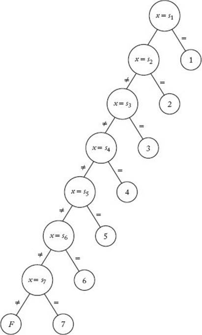
As we did for deterministic sorting algorithms, we can associate a decision tree with every deterministic algorithm that searches for a key x in an array of n keys. Figure 8.1 shows a decision tree corresponding to Binary Search when searching seven keys, and Figure 8.2 shows a decision tree corresponding to Sequential Search (Algorithm 1.1). In these trees, each large node represents a comparison of an array item with the search key x, and each small node (leaf) contains a result that is reported. When x is in the array, we report an index of the item that it equals, and when x is not in the array, we report an “F” for failure. In Figures 8.1 and 8.2, s1 through s7 are the values such that
Figure 8.1 The decision tree corresponding to Binary Search when searching seven keys.
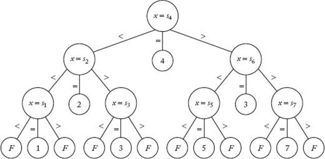
Figure 8.2 The decision tree corresponding to Sequential Search when searching seven keys.
![]()
We assume that a searching algorithm never changes any array values, so these are still the values after the search is completed.
Each leaf in a decision tree for searching n keys for a key x represents a point at which the algorithm stops and reports an index i such that x = si or reports failure. Every internal node represents a comparison. A decision tree is called valid for searching n keys for a key x if for each possible outcome there is a path from the root to a leaf that reports that outcome. That is, there must be paths for x = si for 1 ≤ i ≤ n and a path that leads to failure. The decision tree is called pruned if every leaf is reachable. Every algorithm that searches for a key x in an array of n keys has a corresponding pruned, valid decision tree. In general, a searching algorithm need not always compare x with an array item. That is, it could compare two array items. However, because we are assuming that all keys are distinct, the outcome will be equality only when x is being compared. In the cases of both Binary Search and Sequential Search, when the algorithm determines that x equals an array item, it stops and returns the index of the array item. An inefficient algorithm may continue to do comparisons when it determines that x equals an array item and return the index later. However, we can replace such an algorithm with one that stops at this point and returns the index. The new algorithm will be at least as efficient as the original one. Therefore, we need only consider pruned, valid decision trees for searching n distinct keys for a key x in which equality leads to a leaf that returns an index. Because there are only three possible results of a comparison, a deterministic algorithm can take at most three different paths after each comparison. This means that each comparison node in the corresponding decision tree can have at most three children. Because equality must lead to a leaf that returns an index, at most two of the children can be comparison nodes. Therefore, the set of comparison nodes in the tree constitutes a binary tree. See the sets of large nodes in Figures 8.1 and 8.2 for examples.
• 8.1.1 Lower Bounds for Worst-Case Behavior
Because every leaf in a pruned, valid decision tree must he reachable, the worst-case number of comparisons done by such a tree is the number of nodes in the longest path from the root to a leaf in the binary tree consisting of the comparison nodes. This number is the depth of the binary tree plus 1. Therefore, to establish a lower bound on the worst-case number of comparisons, we need only establish a lower bound on the depth of the binary tree consisting of the comparison nodes. Such a bound is established by means of the following lemmas and theorem.
![]() Lemma 8.1
Lemma 8.1
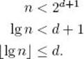
If n is the number of nodes in a binary tree and d is the depth, then
![]()
Proof: We have
![]()
because there can be only one root, at most two nodes with depth 1, 22 nodes with depth 2, … , and 2d nodes with depth d. Applying the result in Example A.3 in Appendix A yields
![]()
which means that
Although the next lemma seems obvious, it is not easy to prove rigorously.
![]() Lemma 8.2
Lemma 8.2
To be a pruned, valid decision tree for searching n distinct keys for a key x, the binary tree consisting of the comparison nodes must contain at least n nodes.
Proof: Let si for 1 ≤ i ≤ n be the values of the n keys. First we show that every si must be in at least one comparison node (that is, it must be involved in at least one comparison). Suppose that for some i this is not the case. Take two inputs that are identical for all keys except the ith key and are different for the ith key. Let x have the value of si in one of the inputs. Because si is not involved in any comparisons and all the other keys are the same in both inputs, the decision tree must behave the same for both inputs. However, it must report i for one of the inputs, and it must not report i for the other. This contradiction shows that every si must be in at least one comparison node.
Because every si must be in at least one comparison node, the only way we could have less than n comparison nodes would be to have at least one key si involved only in comparisons with other keys—that is, one si that is never compared with x. Suppose we do have such a key. Take two inputs that are equal everywhere except for si, with si being the smallest key in both inputs. Let x be the ith key in one of the inputs. A path from a comparison node containing si must go in the same direction for both inputs, and all the other keys are the same in both inputs. Therefore, the decision tree must behave the same for the two inputs. However, it must report i for one of them and must not report i for the other. This contradiction proves the lemma.
![]() Theorem 8.1
Theorem 8.1
Any deterministic algorithm that searches for a key x in an array of n distinct keys only by comparisons of keys must in the worst case do at least
![]()
Proof: Corresponding to the algorithm, there is a pruned, valid decision tree for searching n distinct keys for a key x. The worst-case number of comparisons is the number of nodes in the longest path from the root to a leaf in the binary tree consisting of the comparison nodes in that decision tree. This number is the depth of the binary tree plus 1. Lemma 8.2 says that this binary tree has at least n nodes. Therefore, by Lemma 8.1, its depth is greater than or equal to ![]() lg n
lg n![]() . This proves the theorem.
. This proves the theorem.
Recall from Section 2.1 that the worst-case number of comparisons done by Binary Search is ![]() lg n
lg n![]() + 1. Therefore, Binary Search is optimal as far as its worst-case performance is concerned.
+ 1. Therefore, Binary Search is optimal as far as its worst-case performance is concerned.
• 8.1.2 Lower Bounds for Average-Case Behavior
Before discussing bounds for the average case, let’s do an average-case analysis of Binary Search. We have waited until now to do this analysis because the use of the decision tree facilitates the analysis. First we need a definition and a lemma.
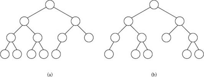
A binary tree is called a nearly complete binary tree if it is complete down to a depth of d − 1. Every essentially complete binary tree is nearly complete, but not every nearly complete binary tree is essentially complete, as illustrated in Figure 8.3. (See Section 7.6 for definitions of complete and essentially complete binary trees.)
Like Lemma 8.2, the following lemma appears to be obvious but is not easy to prove rigorously.
![]() Lemma 8.3
Lemma 8.3
The tree consisting of the comparison nodes in the pruned, valid decision tree corresponding to Binary Search is a nearly complete binary tree.
Proof: The proof is done by induction on n, the number of keys. Clearly, the tree consisting of the comparison nodes is a binary tree containing n nodes, one for each key. Therefore, we can do the induction on the number of nodes in this binary tree.
Figure 8.3 (a) An essentially complete binary tree. (b) A nearly complete but not essentially complete binary tree.
Induction base: A binary tree containing one node is nearly complete.
Induction hypothesis: Assume that for all k < n the binary tree containing k nodes is nearly complete.
Induction step: We need to show that the binary tree containing n nodes is nearly complete. We do this separately for odd and even values of n.
If n is odd, the first split in Binary Search splits the array into two sub-arrays each of size (n − 1/2). Therefore, both the left and right subtrees are the binary tree corresponding to Binary Search when searching (n − 1) /2 keys, which means that, as far as structure is concerned, they are the same tree. They are nearly complete, by the induction hypothesis. Because they are the same nearly complete tree, the tree in which they are the left and right subtrees is nearly complete.
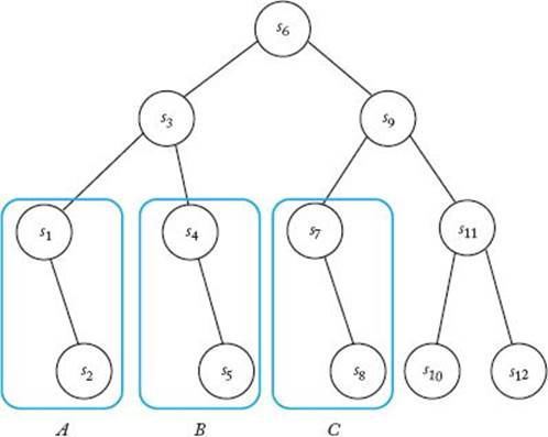
If n is even, the first split in Binary Search splits the array into a subarray of size n/2 on the right and a subarray of size (n/2) − 1 on the left. To enable us to speak concretely, we will discuss the case in which the odd number of keys is on the left. The proof is analogous when the odd number of keys is on the right. When the odd number is on the left, the left and right subtrees of the left subtree are the same tree (as discussed previously). One subtree of the right subtree is also that same tree (you should verify this). Because the right subtree is nearly complete (by the induction hypothesis) and because one of its subtrees is the same tree as the left and right subtrees of the left subtree, the entire tree must be nearly complete. See Figure 8.4 for an illustration.
Figure 8.4 The binary tree consisting of the comparison nodes in the decision tree corresponding to Binary Search when n = 12. Only the vaIues of the keys are shown at the nodes. Subtrees A, B, and C all have the same structure.
We can now do an average-case analysis of Binary Search.
Analysis of Algorithm 8.1
![]() Average-Case Time CompIexity (Binary Search, Recursive)
Average-Case Time CompIexity (Binary Search, Recursive)
Basic operation: the comparison of x with S [mid].
Input size: n, the number of items in the array.
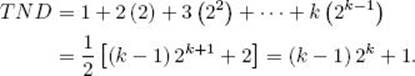
First, we analyze the case in which we know that x is in the array. We do this analysis under the assumption that x is equally likely to be in each of the array slots. Let’s call the total number of nodes in the path from the root to a node the node distance to that node, and the sum of the node distances to all nodes the total node distance (TND) of a tree. Notice that the distance to a node is 1 greater than the length of the path from the root to the node. For the binary tree consisting of the comparison nodes in Figure 8.1,
![]()
It is not hard to see that the total number of comparisons done by Binary Search’s decision tree to locate x at all possible array slots is equal to the TND of the binary tree consisting of the comparison nodes in that decision tree. Given the assumption that all slots are equally probable, the average number of comparisons required to locate x is therefore TND/n. For simplicity, let’s initially assume that n = 2k − 1 for some integer k. Lemma 8.3 says that the binary tree consisting of the comparison nodes in the decision tree corresponding to Binary Search is nearly complete. It is not hard to see that if a nearly complete binary tree contains 2k − 1 nodes, it is a complete binary tree. The binary tree consisting of the comparison nodes in Figure 8.1 illustrates the case in which k = 3. In a complete binary tree, the TND is given by
The second-to-last equality is obtained by applying the result from Example A.5 in Appendix A. Because 2k = n + 1, the average number of comparisons is given by
![]()
For n in general, the average number of comparisons is bounded approximately by
![]()
The average is near the lower bound if n is a power of 2 or is slightly greater than a power of 2, and the average is near the upper bound if n is slightly smaller than a power of 2. You are shown how to establish this result in the exercises. Intuitively, Figure 8.1 shows why this is so. If we add just one node so that the total number of nodes is 8, ![]() lg n
lg n![]() jumps from 2 to 3, but the average number of comparisons hardly changes.
jumps from 2 to 3, but the average number of comparisons hardly changes.
Next, we analyze the case in which x may not be in the array. There are 2n + 1 possibilities: x could be less than all the items, between any two of the items, or greater than all the items. That is, we could have
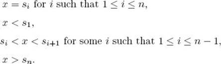
We analyze the case in which each of these possibilities is equally likely. For simplicity, we again initially assume that n = 2k − 1 for some integer k. The total number of comparisons for the successful searches is the TND of the binary tree consisting of the comparison nodes. Recall that this number equals (k − 1) 2k + 1. There are k comparisons for each of the n + 1 unsuccessful searches (see Figure 8.1). The average number of comparisons is therefore given by
![]()
Because 2k = n + 1, we have
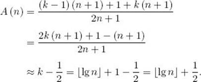
For n in general, the average number of comparisons is bounded approximately by
![]()
The average is near the lower bound if n is a power of 2 or is slightly greater than a power of 2, and the average is near the upper bound if n is slightly smaller than a power of 2. You are asked to establish this result in the exercises.
Binary Search’s average-case performance is not much better than its worst case. We can see why this is so by looking again at Figure 8.1. In that figure, there are more result nodes at the bottom of the tree (where the worst case occurs) than there are in the rest of the tree. This is true even if we don’t consider unsuccessful searches. (Notice that all of the unsuccessful searches are at the bottom of the tree.)
Next we prove that Binary Search is optimal in the average case given the assumptions in the previous analysis. First, we define minTND(n) as the minimum of the TND for binary trees containing n nodes.
![]() Lemma 8.4
Lemma 8.4
The TND of a binary tree containing n nodes is equal to minTND (n) if and only if the tree is nearly complete.
Proof: First we show that if a tree’s TND = minTND (n), the tree is nearly complete. To that end, suppose that some binary tree is not nearly complete. Then there must be some node, not at one of the bottom two levels, that has at most one child. We can remove any node A from the bottom level and make it a child of that node. The resulting tree will still be a binary tree containing n nodes. The number of nodes in the path to A in that tree will be at least 1 less than the number of nodes in the path to A in the original tree. The number of nodes in the paths to all other nodes will be the same. Therefore, we have created a binary tree containing n nodes with a TND smaller than that of our original tree, which means that our original tree did not have a minimum TND.
It is not hard to see that the TND is the same for all nearly complete binary trees containing n nodes. Therefore, every such tree must have the minimum TND.
![]() Lemma 8.5
Lemma 8.5
Suppose that we are searching n keys, the search key x is in the array, and all array slots are equally probable. Then the average-case time complexity for Binary Search is given by
![]()
Proof: As discussed in the average-case analysis of Binary Search, the average-case time complexity is obtained by dividing by n the TND of the binary tree consisting of the comparison nodes in its corresponding decision tree. The proof follows from Lemmas 8.3 and 8.4.
![]() Lemma 8.6
Lemma 8.6
If we assume that x is in the array and that all array slots are equally probable, the average-case time complexity of any deterministic algorithm that searches for a key x in an array of n distinct keys is bounded below by
![]()
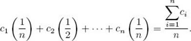
Proof: As shown in Lemma 8.2, every array item si must be compared with x at least once in the decision tree corresponding to the algorithm. Let ci be the number of nodes in the shortest path to a node containing a comparison of si with x. Because each key has the same probability 1/n of being the search key x, a lower bound on the average-case time complexity is given by
It is left as an exercise to show that the numerator in this last expression is greater than or equal to minTND (n).
![]() Theorem 8.2
Theorem 8.2
Among deterministic algorithms that search for a key x in an array of n distinct keys only by comparison of keys, Binary Search is optimal in its average-case performance if we assume that x is in the array and that all array slots are equally probable. Therefore, under these assumptions, any such algorithm must on the average do at least approximately
![]()
Proof: The proof follows from Lemmas 8.5 and 8.6 and the average-case time complexity analysis of Binary Search.
It is also possible to show that Binary Search is optimal in its average-case performance if we assume that all 2n+1 possible outcomes (as discussed in the average-case analysis of Binary Search) are equally likely.
We established that Binary Search is optimal in its average-case performance given specific assumptions about the probability distribution. For other probability distributions, it may not be optimal. For example, if the probability was 0.9999 that x equaled S [1], it would be optimal to compare xwith S [1] first. This example is a bit contrived. A more real-life example would be a search for a name picked at random from people in the United States. As discussed in Section 3.5, we would not consider the names “Tom” and “Ursula” to be equally probable. The analysis done here is not applicable, and other considerations are needed. Section 3.5 addresses some of these considerations.
8.2 Interpolation Search
The bounds just obtained are for algorithms that rely only on comparisons of keys. We can improve on these bounds if we use some other information to assist in our search. Recall that Barney Beagle does more than just compare keys to find Colleen Collie’s number in the phone book. He does not start in the middle of the phone book, because he knows that the C’s are near the front. He “interpolates” and starts near the front. We develop an algorithm for this strategy next.
Suppose we are searching 10 integers, and we know that the first integer ranges from 0 to 9, the second from 10 to 19, the third from 20 to 29, … , and the tenth from 90 to 99. Then we can immediately report failure if the search key x is less than 0 or greater than 99, and, if neither of these is the case, we need only compare x with S [1 + ![]() x/10
x/10![]() ]. For example, we would compare x = 25 with S [1 +
]. For example, we would compare x = 25 with S [1 + ![]() 25/10
25/10![]() ] = S [3]. If they were not equal, we would report failure.
] = S [3]. If they were not equal, we would report failure.
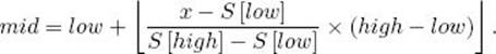
We usually do not have this much information. However, in some applications it is reasonable to assume that the keys are close to being evenly distributed between the first one and the last one. In such cases, instead of checking whether x equals the middle key, we can check whether x equals the key that is located about where we would expect to find x. For example, if we think 10 keys are close to being evenly distributed from 0 to 99, we would expect to find x = 25 about in the third position, and we would compare x first with S [3] instead of S [5]. The algorithm that implements this strategy is called Interpolation Search. As in Binary Search, low is set initially to 1 and high to n. We then use linear interpolation to determine approximately where we feel x should be located. That is, we compute
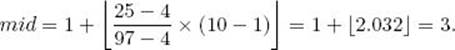
For example, if S [1] = 4 and S [10] = 97, and we were searching for x = 25,
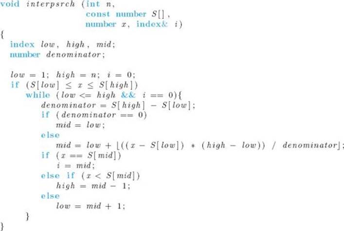
Other than the different way of computing mid and some extra book-keeping, the Interpolation Search algorithm proceeds like Binary Search (Algorithm 1.5).
![]() Algorithm 8.1
Algorithm 8.1
Interpolation Search
Problem: Determine whether x is in the sorted array S of size n.
Inputs: positive integer n, and sorted (nondecreasing order) array of numbers S indexed from 1 to n.
Outputs: the location i of x in S; 0 if x is not in S.
If the keys are close to being evenly spaced, Interpolation Search homes in on the possible location of x more quickly than does Binary Search. For instance, in the preceding example, if x = 25 were less than S [3], Interpolation Search would reduce the instance of size 10 to one of size 2, whereas Binary Search would reduce it to one of size 4.
Suppose that the keys are uniformly distributed between S [1] and S [n]. By this we mean that the probability of a randomly chosen key being in a particular range equals its probability of being in any other range of the same length. If this were the case, we would expect to find x at approximately the slot determined by Interpolation Search, and therefore we would expect Interpolation Search to outperform Binary Search on the average. Indeed, under the assumptions that the keys are uniformly distributed and that the search key x is equally likely to be in each of the array slots, it is possible to show that the average-case time complexity of Interpolation Search is given by
![]()
If n equals one billion, lg (lg n) is about 5, whereas lg n is about 30.
A drawback of Interpolation Search is its worst-case performance. Suppose again that there are 10 keys and their values are 1, 2, 3, 4, 5, 6, 7, 8, 9, and 100. If x were 10; mid would repeatedly be set to low, and x would be compared with every key. In the worst case, Interpolation Search degenerates to a sequential search. Notice that the worst case happens when mid is repeatedly set to low. A variation of Interpolation Search called Robust Interpolation Search remedies this situation by establishing a variable gap such that mid − low and high − mid are always greater than gap. Initially we set
![]()
and we compute mid using the previous formula for linear interpolation. After that computation, the value of mid is possibly changed with the following computation:
![]()
In the example where x = 10 and the 10 keys are 1, 2, 3, 4, 5, 6, 7, 8, 9, and 100, gap would initially be ![]() mid would initially be 1, and we would obtain
mid would initially be 1, and we would obtain
![]()
In this way we guarantee that the index used for the comparison is at least gap positions away from low and high. Whenever the search for x continues in the subarray containing the larger number of array elements, the value of gap is doubled, but it is never made greater than half the number of array elements in that subarray. For instance, in the previous example, the search for x continues in the larger subarray (the one from S [5] to S [10]). Therefore, we would double gap, except that in this case the subarray contains only six array elements, and doubling gap would make it exceed half the number of array elements in the subarray. We double gap in order to quickly escape from large clusters. When x is found to lie in the subarray containing the smaller number of array elements, we reset gap to its initial value.
Under the assumptions that the keys are uniformly distributed and that the search key x is equally likely to be in each of the array slots, the average-case time complexity for Robust Interpolation Search is in Θ(lg(lg n)). Its worst-case time complexity is in Θ((lg n)2), which is worse than Binary Search but much better than Interpolation Search.
There are quite a few extra computations in Robust Interpolation Search relative to Interpolation Search and in Interpolation Search relative to Binary Search. In practice, one should analyze whether the savings in comparisons justifies this increase in computations.
The searches described here are also applicable to words, because words can readily be encoded as numbers. We can therefore apply the modified binary search method to searching the phone book.
8.3 Searching in Trees
We next discuss that even though Binary Search and its variations, Interpolation Search and Robust Interpolation Search, are very efficient, they cannot be used in many applications because an array is not an appropriate structure for storing the data in these applications. Then we show that a tree is appropriate for these applications. Furthermore, we show that we have Θ (lg n) algorithms for searching trees.
By static searching we mean a process in which the records are all added to the file at one time and there is no need to add or delete records later. An example of a situation in which static searching is appropriate is the searching done by operating systems commands. Many applications, however, require dynamic searching, which means that records are frequently added and deleted. An airline reservation system is an application that requires dynamic searching, because customers frequently call to schedule and cancel reservations.
An array structure is inappropriate for dynamic searching, because when we add a record in sequence to a sorted array, we must move all the records following the added record. Binary Search requires that the keys be structured in an array, because there must be an efficient way to find the middle item. This means that Binary Search cannot be used for dynamic searching. Although we can readily add and delete records using a linked list, there is no efficient way to search a linked list. Therefore, linked lists do not satisfy the searching needs of a dynamic searching application. If it is necessary to retrieve the keys quickly in sorted sequence, direct-access storage (hashing) will not work (hashing is discussed in the next section). Dynamic searching can be implemented efficiently using a tree structure. First we discuss binary search trees. After that, we discuss B-trees, which are an improvement on binary search trees. B-trees are guaranteed to remain balanced.
Our purpose here is to further analyze the problem of searching. Therefore, we only touch on the algorithms pertaining to binary search trees and B-trees. These algorithms are discussed in detail in many data structures texts, such as Kruse (1994).
• 8.3.1 Binary Search Trees
Binary search trees were introduced in Section 3.5. However, the purpose there was to discuss a static searching application. That is, we wanted to create an optimal tree based on the probabilities of searching for the keys. The algorithm that builds the tree (Algorithm 3.9) requires that all the keys be added at one time, which means that the application requires static searching. Binary search trees are also appropriate for dynamic searching. Using a binary search tree, we can usually keep the average search time low, while being able to add and delete keys quickly. Furthermore, we can quickly retrieve the keys in sorted sequence by doing an in-order traversal of the tree. Recall that in an in-order traversal of a binary tree, we traverse the tree by first visiting all the nodes in the left subtree using an in-order traversal, then visiting the root, and finally visiting all the nodes in the right subtree using an in-order traversal.
Figure 8.5 shows a binary search tree containing the first seven integers. The search algorithm (Algorithm 3.8) searches the tree by comparing the search key x with the value at the root. If they are equal, we are done. If x is smaller, the search strategy is applied to the left child. If x is larger, the strategy is applied to the right child. We proceed down the tree in this fashion until x is found or it is determined that x is not in the tree. You may have noticed that when we apply this algorithm to the tree in Figure 8.5, we do the same sequence of comparisons as done by the decision tree (seeFigure 8.1) corresponding to Binary Search. This illustrates a fundamental relationship between Binary Search and binary search trees. That is, the comparison nodes in the decision tree, corresponding to Binary Search when searching n keys, also represent a binary search tree in which Algorithm 3.8 does the same comparisons as Binary Search. Therefore, like Binary Search, Algorithm 3.8 is optimal for searching n keys when it is applied to that tree.
We can efficiently add keys to and delete keys from the tree in Figure 8.5. For example, to add the key 5.5 we simply proceed down the tree, going to the right if 5.5 is greater than the key at a given node, and to the left otherwise, until we locate the leaf containing 5. We then add 5.5 as the right child of that leaf. As previously mentioned, the actual algorithms for adding and deleting can be found in Kruse (1994).
Figure 8.5 A binary search tree containing the first seven integers.
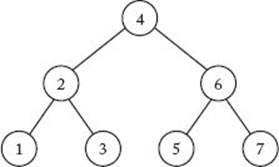
Figure 8.6 A skewed binary search tree containing the first seven integers.
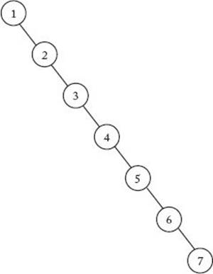
The drawback of binary search trees is that when keys are dynamically added and deleted, there is no guarantee that the resulting tree will be balanced. For example, if the keys are all added in increasing sequence, we obtain the tree in Figure 8.6. This tree, which is called a skewed tree, is simply a linked list. An application of Algorithm 3.8 to this tree results in a sequential search. In this case, we have gained nothing by using a binary search tree instead of a linked list.
If the keys are added at random, intuitively it seems that the resulting tree will be closer to a balanced tree much more often than it will be closer to a linked list. (See Section A.8.1. in Appendix A for a discussion of randomness.) Therefore, on the average, we would expect an efficient search time. Indeed, we have a theorem to that effect. First we explain the result in the theorem. The theorem obtains an average search time for inputs containing n keys under the assumption that all inputs are equally probable. By this we mean that every possible ordering of n keys has the same probability of being the input to the algorithm that builds the tree. For example, if n = 3 and s1 < s2 < s3 are the three keys. these inputs are all equally probable:
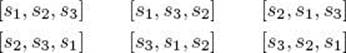
Notice that two inputs can result in the same tree. For example, [s2, s3, s1] and [s2, s1, s3] result in the same tree—namely, the one with s2 at the root, s1 on the left, and s3 on the right. These are the only two inputs that produce that tree. Sometimes a tree is produced by only one input. For example, the tree produced by the input [s1, s2, s3] is produced by no other input. It is the inputs, not the trees, that are assumed to he equiprobable. Therefore, each of the inputs listed has probability ![]() , the tree produced by the inputs [s2, s3, s1] and [s2, s1, s3] has probability ⅓ , and the tree produced by the input [s1, s2, s3] has probability
, the tree produced by the inputs [s2, s3, s1] and [s2, s1, s3] has probability ⅓ , and the tree produced by the input [s1, s2, s3] has probability ![]() . We also assume that the search key x is equally probable to be any of the n keys. The theorem now follows.
. We also assume that the search key x is equally probable to be any of the n keys. The theorem now follows.
![]() Theorem 8.3
Theorem 8.3
Under the assumptions that all inputs are equally probable and that the search key x is equally probable to be any of the n keys, the average search time over all inputs containing n distinct keys, using binary search trees, is given approximately by
![]()
Proof: We obtain the proof under the assumption that the search key x is in the tree. In the exercises, we show that the result still holds if we remove this restriction, as long as we consider each of the 2n + 1 possible outcomes to be equally probable. (These outcomes are discussed in the average-case analysis of Binary Search in Section 8.1.2.)
Consider all binary search trees containing n keys that have the kth-smallest key at the root. Each of these trees has k − 1 nodes in its left subtree and n − k nodes in its right subtree. The average search time for the inputs that produce these trees is given by the sum of the following three quantities:
• The average search time in the left subtrees of such trees times the probability of x being in the left subtree
• The average search time in the right subtrees of such trees times the probability of x being in the right subtree
• The one comparison at the root
The average search time in the left subtrees of such trees is A (k − 1), and the average search time in the right subtrees is A (n − k). Because we have assumed that the search key x is equally probable to be any of the keys, the probabilities of x being in the left and right subtrees are, respectively,
![]()
If we let A (n|k) denote the average search time over all inputs of size n that produce binary search trees with the kth-smallest key at the root, we have established that
![]()
Because all inputs are equally probable, every key has the same probability of being the first key in the input and therefore the key at the root. Therefore, the average search time over all inputs of size n is the average of A (n|k) as k goes from 1 to n. We have then
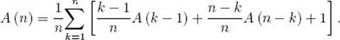
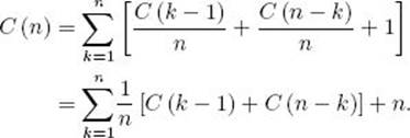
If we set C (n) = nA (n) and substitute C (n) /n in the expression for A (n), we obtain
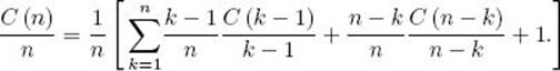
Simplifying yields
The initial condition is
![]()
This recurrence is almost identical to the one for the average case of Quicksort (Algorithm 2.6). Mimicking the average-case analysis for Quicksort yields
![]()
which means that
![]()
You must be careful not to misinterpret the result in Theorem 8.3. This theorem does not mean that the average search time for a particular input containing n keys is about 1.38 lg n. A particular input could produce a tree that degenerates into the one in Figure 8.6, which means that the average search time is in Θ (n). Theorem 8.3 is for the average search time over all inputs containing n keys. Therefore, for any given input containing n keys, it is probable that the average search time is in Θ (lg n) but it could be in Θ (n). There is no guarantee of an efficient search.
• 8.3.2 B-Trees
In many applications, performance can be severely degraded by a linear search time. For example, the keys to records in large databases often cannot all fit in a computer’s high-speed memory (called “RAM,” for “random access memory”) at one time. Therefore, multiple disk accesses are needed to accomplish the search. (Such a search is called an external search, whereas when all the keys are simultaneously in memory it is called an internal search.) Because disk access involves the mechanical movement of read/write heads and RAM access involves only electronic data transfer, disk access is orders of magnitude slower than RAM access. A linear-time external search could therefore prove to be unacceptable, and we would not want to leave such a possibility to chance.
One solution to this dilemma is to write a balancing program that takes as input an existing binary search tree and outputs a balanced binary search tree containing the same keys. The program is then run periodically. Algorithm 3.9 is an algorithm for such a program. That algorithm is more powerful than a simple balancing algorithm because it is able to consider the probability of each key being the search key.
In a very dynamic environment, it would be better if the tree never became unbalanced in the first place. Algorithms for adding and deleting nodes while maintaining a balanced binary tree were developed in 1962 by two Russian mathematicians, G. M. Adel’son-Vel’skii and E. M. Landis. (For this reason, balanced binary trees are often called AVL trees.) These algorithms can be found in Kruse (1994). The addition and deletion times for these algorithms are guaranteed to be Θ (lg n), as is the search time.
In 1972, R. Bayer and E. M. McCreight developed an improvement over binary search trees called B-trees. When keys are added to or deleted from a B-tree, all leaves are guaranteed to remain at the same level, which is even better than maintaining balance. The actual algorithms for manipulating B-trees can be found in Kruse (1994). Here we illustrate only how we can add keys while keeping all leaves at the same level.
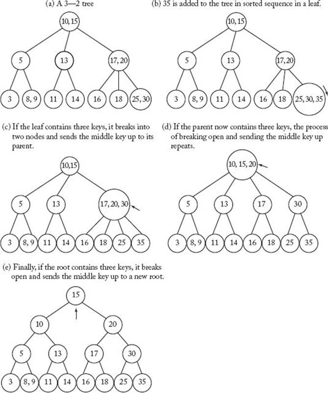
B-trees actually represent a class of trees, of which the simplest is a 3–2 tree. We illustrate the process of adding nodes to such trees. A 3–2 tree is a tree with the following properties:
• Each node contains one or two keys.
• If a nonleaf contains one key, it has two children, whereas if it contains two keys, it has three children.
• The keys in the left subtree of a given node are less than or equal to the key stored at that node.
• The keys in the right subtree of a given node are greater than or equal to the key stored at that node.
• If a node contains two keys, the keys in the middle subtree of the node are greater than or equal to the left key and less than or equal to the right key.
• All leaves are at the same level.
Figure 8.7(a) shows a 3–2 tree, and the remainder of that figure shows how a new key is added to the tree. Notice that the tree remains balanced because the tree grows in depth at the root instead of at the leaves. Similarly, when it is necessary to delete a node, the tree shrinks in depth at the root. In this way, all leaves always remain at the same level, and the search, addition, and deletion times are guaranteed to be in Θ (lg n). Clearly, an in-order traversal of the tree retrieves the keys in sorted sequence. For these reasons, B-trees are used in most modern database management systems.
Figure 8.7 The way a new key is added to a
8.4 Hashing
Suppose the keys are integers from 1 to 100, and there are about 100 records. An efficient method for storing the records is to create an array S of 100 items and store the record whose key is equal to i in S [i]. The retrieval is immediate, with no comparisons of keys being done. This same strategy can be used if there are about 100 records and the keys are nine-digit social security numbers. However, in this case the strategy is very inefficient in terms of memory because an array of 1 billion items is needed to store only 100 records. Alternatively, we could create an array of only 100 items indexed from 0 to 99, and “hash” each key to a value from 0 and 99. A hash function is a function that transforms a key to an index, and an application of a hash function to a particular key is called “hashing the key.” In the case of social security numbers, a possible hash function is
![]()
(% returns the remainder when key is divided by 100.) This function simply returns the last two digits of the key. If a particular key hashes to i, we store the key and its record at S [i]. This strategy does not store the keys in sorted sequence, which means that it is applicable only if we never need to retrieve the records efficiently in sorted sequence. If it is necessary to do this, one of the methods discussed previously should be used.
If no two keys hash to the same index, this method works fine. However, this is rarely the case when there are a substantial number of keys. For example, if there are 100 keys and each key is equally likely to hash to each of the 100 indices, the probability of no two keys hashing to the same index is
![]()
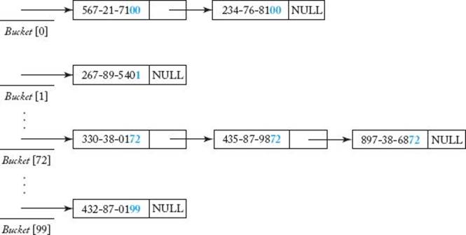
We are almost certain that at least two keys will hash to the same index. Such an occurrence is called a collision or hash clash. There are various ways to resolve a collision. One of the best ways is through the use of open hashing (also called open addressing). With open hashing we create a bucket for each possible hash value and place all the keys that hash to a value in the bucket associated with that value. Open hashing is usually implemented with linked lists. For example, if we hash to the last two digits of a number, we create an array of pointers Bucket that is indexed from 0 to 99. All of those keys that hash to i are placed in a linked list starting at Bucket [i]. This is illustrated in Figure 8.8.
Figure 8.8 An illustration of open hashing. Keys with the same last two digits are in the same bucket.
The number of buckets need not equal the number of keys. For example, if we hash to the last two digits of a number, the number of buckets must be 100. However, we could store 100, 200, 1000, or any number of keys. Of course, the more keys we store, the more likely we are to have collisions. If the number of keys is greater than the number of buckets, we are guaranteed to have collisions. Because a bucket stores only a pointer, not much space is wasted by allocating a bucket. Therefore, it is often reasonable to allocate at least as many buckets as there are keys.
When searching for a key, it is necessary to do a sequential search through the bucket (linked list) containing the key. If all the keys hash to the same bucket, the search degenerates into a sequential search. How likely is this to happen? If there are 100 keys and 100 buckets, and a key is equally likely to hash to each of the buckets, the probability of the keys all ending up in the same bucket is
Therefore, it is almost impossible for all the keys to end up in the same bucket. What about the chances of 90, 80, 70, or any other large number of keys ending up in the same bucket? Our real interest should be how likely it is that hashing will yield a better average search than Binary Search. We show that if the file is reasonably large, this too is almost a certainty. But first we show how good things can be with hashing.
Intuitively, it should be clear that the best thing that can happen is for the keys to be uniformly distributed in the buckets. That is, if there are n keys and m buckets, each bucket contains n/m keys. Actually, each bucket will contain exactly n/m keys only when n is a multiple of m. When this is not the case, we have an approximately uniform distribution. The following theorems show what happens when the keys are uniformly distributed. For simplicity, they are stated for an exact uniform distribution (that is, for the case in which n is a multiple of m).
![]() Theorem 8.4
Theorem 8.4
If n keys are uniformly distributed in m buckets, the number of comparisons in an unsuccessful search is given by n/m.
Proof: Because the keys are uniformly distributed, the number of keys in each bucket is n/m, which means that every unsuccessful search requires n/m comparisons.
![]() Theorem 8.5
Theorem 8.5
If n keys are uniformly distributed in m buckets and each key is equally likely to be the search key, the average number of comparisons in a successful search is given by
![]()
Proof: The average search time in each bucket is equal to the average search time when doing a sequential search of n/m keys. The average-case analysis of Algorithm 1.1 in Section 1.3 shows that this average equals the expression in the statement of the theorem.
The following example applies Theorem 8.5.
Example 8.1
If the keys are uniformly distributed and n = 2m, every unsuccessful search requires only 2m/m = 2 comparisons, and the average number of comparisons for a successful search is
![]()
When the keys are uniformly distributed, we have a very small search time. However, even though hashing has the possibility of yielding such exceptionally good results, one might argue that we should still use Binary Search to guarantee that the search does not degenerate into something close to a sequential search. The following theorem shows that if the file is reasonably large, the chances of hashing being as bad as Binary Search are very small. The theorem assumes that a key is equally likely to hash to each of the buckets. When social security numbers are hashed to their last two digits, this criterion should be satisfied. However, not all hash functions satisfy this criterion. For example, if names are hashed to their last letters, the probability of hashing to “th” is much greater than that of hashing to “qz,” because many more names end in “th.” A data structures text such as Kruse (1994) discusses methods for choosing a good hash function. Our purpose here is to analyze how well hashing solves the Searching problem.
![]() Theorem 8.6
Theorem 8.6
If there are n keys and m buckets, the probability that at least one bucket contains at least k keys is less than or equal to
given the assumption that a key is equally likely to hash to any bucket.
Proof: For a given bucket, the probability of any specific combination of k keys ending up in that bucket is (1/m)k, which means that the probability that the bucket contains at least the keys in that combination is (1/m)k. In general, for two events S and T ,
![]()
Therefore, the probability that a given bucket contains at least k keys is less than or equal to the sum of the probabilities that it contains at least the keys in each distinct combination of k keys. Because (n k)distinct combinations of k keys can be obtained from n keys (see Section A.7 in Appendix A), the probability that any given bucket contains at least k keys is less than or equal to
The theorem now follows from Expression 8.1 and the fact that there are m buckets.
Recall that the average search time for Binary Search is about lg n. Table 8.1 shows the bounds on the probabilities of at least one bucket containing at least lg n keys and 2 lg n keys for several values of n. It is assumed in the table that n = m. Even when n is only 128, the chances of the search time ever exceeding 2 lg n are less than 1 in a billion. For n = 1024, the chances of the search time ever exceeding 2 lg n are less than 3 in 10 million billion. For n = 65, 536, the chances of the search time ever exceeding lg n are about 3 in 1 billion. The probability of dying in a single trip in a jet plane is about 6 in 1 million, and the probability of dying in an auto accident during an average year of driving is about 270 in 1 million. Yet many humans do not take serious measures to avoid these activities. The point is that, to make reasonable decisions, we often neglect exceptionally small probabilities as if they were impossibilities. Because for large n we can be almost certain of obtaining better performance using hashing instead of Binary Search, it is reasonable to do so. We amusingly recall that in the 1970s a certain computer manufacturer routinely talked data-processing managers into buying expensive new hardware by describing a catastrophe that would take place if a contrived scenario of usage occurred. The flaw in their argument, which the data-processing managers often overlooked, was that the probability of this scenario occurring was negligible. Risk aversion is a matter of personal preference. Therefore, an exceedingly risk-averse individual may choose not to take a 1-in-a-billion or even a 3-in-10-million-billion chance. However, the individual should not make such a choice without giving serious deliberation to whether such a decision truly models the individual’s attitude toward risk. Methods for doing such an analysis are discussed in Clemen (1991).
• Table 8.1Upper Bounds on the Probability That at Least One Bucket Contains at Least k Keys*
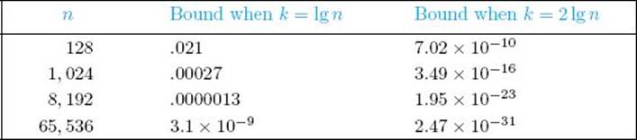
*It is assumed that the number of keys n equals the number of buckets.
8.5 The Selection Problem: Introduction to Adversary Arguments
So far we’ve discussed searching for a key x in a list of n keys. Next we address a different searching problem called the Selection problem. This problem is to find the kth-largest (or kth-smallest) key in a list of n keys. We assume that the keys are in an unsorted array (the problem is trivial for a sorted array). First we discuss the problem for k = 1, which means that we are finding the largest (or smallest) key. Next we show that we can simultaneously find the smallest and largest keys with fewer comparisons than would be necessary if each were found separately. Then we discuss the problem for k = 2, which means that we are finding the second-largest (or second-smallest) key. Finally, we address the general case.
• 8.5.1 Finding the Largest Key
The following is a straightforward algorithm for finding the largest key.
![]() Algorithm 8.2
Algorithm 8.2
Find Largest Key
Problem: Find the largest key in the array S of size n.
Inputs: positive integer n, array of keys S indexed from 1 to n.
Outputs: variable large, whose value is the largest key in S.
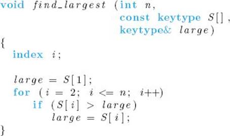
Clearly, the number of comparisons of keys done by the algorithm is given by
![]()
Intuitively, it seems impossible to improve on this performance. The next theorem establishes that this is so. We can think of an algorithm that determines the largest key as a tournament among the keys. Each comparison is a match in the tournament, the larger key is the winner of the comparison, and the smaller key is the loser. The largest key is the winner of the tournament. We use this terminology throughout this section.
![]() Theorem 8.7
Theorem 8.7
Any deterministic algorithm that can find the largest of n keys in every possible input only by comparisons of keys must in every case do at least
![]()
Proof: The proof is by contradiction. That is, we show that if the algorithm does fewer than n − 1 comparisons for some input of size n, the algorithm must give the wrong answer for some other input. To that end, if the algorithm finds the largest key by doing at most n − 2 comparisons for some input, at least two keys in that input never lose a comparison. At least one of those two keys cannot be reported as the largest key. We can create a new input by replacing (if necessary) that key with a key that is larger than all keys in the original input. Because the results of all comparisons will be the same as for the original input, the new key will not be reported as the largest, which means that the algorithm will give the wrong answer for the new input. This contradiction proves that the algorithm must do at least n − 1 comparisons for every input of size n.
You must be careful to interpret Theorem 8.7 correctly. It does not mean that every algorithm that searches only by comparisons of keys must do at least n − 1 comparisons to find the largest key. For example, if an array is sorted, we can find the largest key without doing any comparisons simply by returning the last item in the array. However, an algorithm that returns the last item in an array can find the largest key only when the largest key is the last item. It cannot find the largest key in every possible input. Theorem 8.7 concerns algorithms that can find the largest key in every possible input.
Of course, we can use an analogous version of Algorithm 8.2 to find the smallest key in n − 1 comparisons and an analogous version of Theorem 8.7 to show that n − 1 is a lower bound for finding the smallest key.
• 8.5.2 Finding Both the Smallest and Largest Keys
A straightforward way to find the smallest and largest keys simultaneously is to modify Algorithm 8.2 as follows.
![]() Algorithm 8.3
Algorithm 8.3
Find Smallest and Largest Keys
Problem: Find the smallest and largest keys in an array S of size n.
Inputs: positive integer n, array of keys S indexed from 1 to n.
Outputs: variables small and large, whose values are the smallest and largest keys in S.
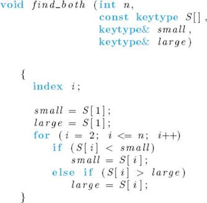
Using Algorithm 8.3 is better than finding the smallest and largest keys independently, because for some inputs the comparison of S [i] with large is not done for every i. Therefore, we have improved on the everycase performance. But whenever S [1] is the smallest key, that comparison is done for all i. Therefore, the worst-ease number of comparisons of keys is given by
![]()
which is exactly the number of comparisons done if the smallest and largest keys are found separately. It may seem that we cannot improve on this performance, but we can. The trick is to pair the keys and find which key in each pair is smaller. This can be done with about n/2 comparisons. We can then find the smallest of all the smaller keys with about n/2 comparisons and the largest of all the larger keys with about n/2 comparisons. In this way, we find both the smallest and largest keys with only about 3n/2 total comparisons. An algorithm for this method follows. The algorithm assumes that n is even.
![]() Algorithm 8.4
Algorithm 8.4
Find Smallest and Largest Keys by Pairing Keys
Problem: Find the smallest and largest keys in an array S of size n.
Inputs: positive even integer n, array of keys S indexed from 1 to n.
Outputs: variables small and large, whose values are the smallest and largest keys in S.
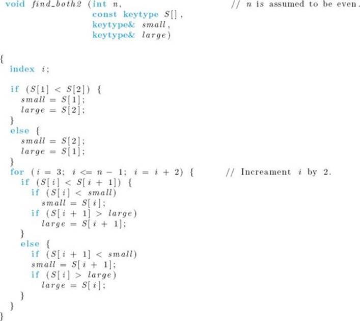
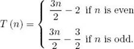
It is left as an exercise to modify the algorithm so that it works when n is odd and to show that its number of comparison of keys is given by
Can we improve on this performance? We show that the answer is “no.” We do not use a decision tree to show this because decision trees do not work well for the Selection problem. The reason is as follows. We know that a decision tree for the Selection problem must contain at least n leaves because there are n possible outcomes. Lemma 7.3 says that if a binary tree has n leaves, its depth is greater than or equal to ![]() lg n
lg n![]() . Therefore, our lower bound on the number of leaves gives us a lower bound of
. Therefore, our lower bound on the number of leaves gives us a lower bound of ![]() lg n
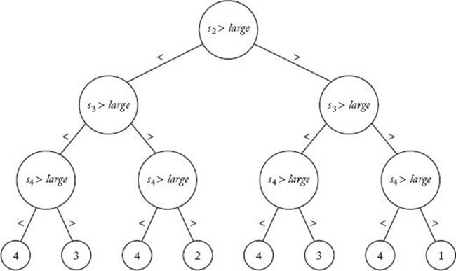
lg n![]() comparisons in the worst case. This is not a very good lower bound, because we already know that it takes at least n − 1 comparisons just to find the largest key (Theorem 8.7). Lemma 8.1 is no more useful because we can only readily establish that there must be n − 1 comparison nodes in the decision tree. Decision trees do not work well for the Selection problem because a result can be in more than one leaf. Figure 8.9 shows the decision tree for Algorithm 8.2 (Find Largest Key) when n = 4. There are four leaves that report 4 and two that report 3. The number of comparisons done by the algorithm is 3 rather than lg n = lg 4 = 2. We see that lg n is a weak lower bound.
comparisons in the worst case. This is not a very good lower bound, because we already know that it takes at least n − 1 comparisons just to find the largest key (Theorem 8.7). Lemma 8.1 is no more useful because we can only readily establish that there must be n − 1 comparison nodes in the decision tree. Decision trees do not work well for the Selection problem because a result can be in more than one leaf. Figure 8.9 shows the decision tree for Algorithm 8.2 (Find Largest Key) when n = 4. There are four leaves that report 4 and two that report 3. The number of comparisons done by the algorithm is 3 rather than lg n = lg 4 = 2. We see that lg n is a weak lower bound.
Figure 8.9 The decision tree corresponding to Algorithm 8.2 when n = 4.
We use another method, called an adversary argument, to establish our lower bound. An adversary is an opponent or foe. Suppose you are in the local singles bar and an interested stranger asked you the tired question, “What’s your sign?” This means that the person wants to know your astrological sign. There are 12 such signs, each corresponding to a period of approximately 30 days. If, for example, you were born August 25, your sign would be Virgo. To make this stale encounter more exciting, you decide to spice things up by being an adversary. You tell the stranger to guess your sign by asking yes/no questions. Being an adversary, you have no intention of disclosing your sign—you simply want to force the stranger to ask as many questions as possible. Therefore, you always provide answers that narrow down the search as little as possible. For example, suppose the stranger asks, “Were you born in summer?” Because a “no” answer would narrow the search to nine months and a “yes” answer would narrow it to three months, you answer “no.” If the stranger then asks, “Were you born in a month with 31 days?” you answer “yes,” because more than half of the nine possible months remaining have 31 days. The only requirement of your answers is that they be consistent with ones already given. For example, if the stranger forgets that you said you were not born in summer and later asks if you were born in July, you could not answer “yes” because this would not be consistent with your previous answers. Inconsistent answers have no sign (birthday) satisfying them. Because you answer each question so as to leave the maximum number of remaining possibilities and because your answers are consistent, you force the stranger to ask as many questions as possible before reaching a logical conclusion.
Suppose some adversary’s goal is to make an algorithm work as hard as possible (as you did with the stranger). At each point where the algorithm must make a decision (for example, after a comparison of keys), the adversary tries to choose a result of the decision that will keep the algorithm going as long as possible. The only restriction is that the adversary must always choose a result that is consistent with those already given. As long as the results are consistent, there must be an input for which this sequence of results occurs. If the adversary forces the algorithm to do the basic instruction f (n) times, then f (n) is a lower bound on the worst-case time complexity of the algorithm.
We use an adversary argument to obtain a lower bound on the worst-case number of comparisons needed to find both the largest and smallest keys. This argument first appeared in Pohl (1972). To establish that bound, we can assume that the keys are distinct. We can do this because a lower bound on the worst-case time complexity for a subset of inputs (those with distinct keys) is a lower bound on the worst-case time complexity when all inputs are considered. Before presenting the theorem, we show our adversary’s strategy. Suppose we have some algorithm that solves the problem of finding the smallest and largest keys only by comparisons of keys. If all the keys are distinct, at any given time during the execution of the algorithm a given key has one of the following states:
|
State |
Description of State |
|
X |
The key has not been involved in a comparison. |
|
L |
The key has lost at least one comparison and has never won. |
|
W |
The key has won at least one comparison and has never lost. |
|
WL |
The key has won at least one comparison and has lost at least one. |
We can think of these states as containing units of information. If a key has state X, there are zero units of information. If a key has state L or W, there is one unit of information because we know that the key has either lost or won a comparison. If a key has state WL, there are two units of information because we know that the key has both won and lost comparisons. For the algorithm to establish that one key small is smallest and another key large is largest, the algorithm must know that every key other than small has won a comparison and every key other than large has lost a comparison. This means that the algorithm must learn
![]()
units of information.
• Table 8.2 Our Adversary’s Strategy for Foiling an Algorithm That Finds the Smallest and Largest Keys*
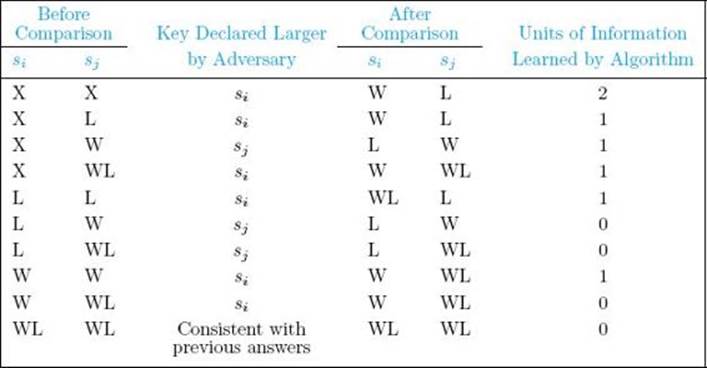
*The keys si and sj are being compared.
Because the goal is to make the algorithm work as hard as possible, an adversary wants to provide as little information as possible with each comparison. For example, if the algorithm first compares s2 and s1, it doesn’t matter what an adversary answers, because two units of information are supplied either way. Let’s say the adversary answers that s2 is larger. The state of s2 then changes from X to W, and the state of s1 changes from X to L. Suppose the algorithm next compares s3 and s1. If an adversary answers that s1 is larger, the state of s1 changes from L to WL and the state of s3changes from X to L. This means that two units of information are disclosed. Because only one unit of information is disclosed by answering that s3 is larger, we have our adversary give this answer. Table 8.2 shows an adversary strategy that always discloses a minimal amount of information. When it doesn’t matter which key is answered, we have simply chosen the first one in the comparison. This strategy is all we need to prove our theorem. But first let’s show an example of how our adversary would actually use the strategy.
Example 8.2
Table 8.3 shows our adversary’s strategy for foiling Algorithm 8.3 for an input size of 5. We have assigned values to the keys that are consistent with the answers. Assigning such values is not really necessary, but the adversary must keep track of the order of the keys imposed by the answers, so that a consistent answer can be given when both keys have state WL. An easy way to do this is to assign values. Furthermore, assigning values illustrates that a consistent set of answers does indeed have an input associated with it. Other than the order determined by the adversary’s strategy, the answers are arbitrary. For example, when s3 is declared larger than s1, we give s3 the value 15. We could have given it any value greater than 10.
• Table 8.3 Our Adversary’s Answers in Attempting to Foil Algorithm 8.3 for an Input Size of 5
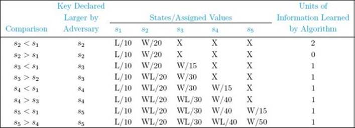
Notice that after s3 is compared with s2, we change the value of s3 from 15 to 30. Remember that the adversary has no actual input when presented with the algorithm. An answer (and therefore an input value) is constructed dynamically whenever our adversary is given the decision the algorithm is currently making. It is necessary to change the value of s3 from 15 because s2 is larger than 15 and our adversary’s answer is that s3 is larger than s2.
After the algorithm is done, s1 has lost to all other keys and s5 has won over all other keys. Therefore, s1 is smallest and s5 is largest. The input constructed by our adversary has s1 as the smallest key because this is an input that makes Algorithm 8.3 work hardest. Notice that eight comparisons are done in Table 8.3, and the worst-case number of comparisons done by Algorithm 8.3 when the input size is 5 is given by
![]()
This means that our adversary succeeds in making Algorithm 8.3 work as hard as possible when the input size is 5.
When presented with a different algorithm for finding the largest and smallest keys, our adversary will provide answers that try to make that algorithm work as hard as possible. You are encouraged to determine the adversary’s answers when presented with Algorithm 8.4 (Find Smallest and Largest Keys by Pairing Keys) and some input size.
When developing an adversary strategy, our goal is to make algorithms for solving some problem work as hard as possible. A poor adversary may not actually achieve this goal. However, regardless of whether or not the goal is reached, the strategy can be used to obtain a lower bound on how hard the algorithms must work. Next we do this for the adversary strategy just described.
![]() Theorem 8.8
Theorem 8.8
Any deterministic algorithm that can find both the smallest and the largest of n keys in every possible input only by comparisons of keys must in the worst case do at least the following numbers of comparisons of keys:
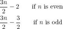
Proof: We show that this is a lower bound on the worst case by showing that the algorithm must do at least this many comparisons when the keys are distinct. As noted previously, the algorithm must learn 2n − 2 units of information to find both the smallest and largest keys. Suppose we present our adversary with the algorithm. Table 8.2 shows that our adversary provides two units of information in a single comparison only when both keys have not been involved in previous comparisons. If n is even, this can be the case for at most
![]()
which means that the algorithm can get at most 2 (n/2) = n units of information in this way. Because our adversary provides at most one unit of information in the other comparisons, the algorithm must do at least
![]()
additional comparisons to get all the information it needs. Our adversary therefore forces the algorithm to do at least
![]()
comparisons of keys. It is left as an exercise to analyze the case in which n is odd.
Because Algorithm 8.4 does the number of comparisons in the bound in Theorem 8.8, that algorithm is optimal in its worst-case performance. We have chosen a worthy adversary because we have found an algorithm that performs as well as the bound it provides. We know therefore that no other adversary could provide a larger bound.
Example 8.2 illustrates why Algorithm 8.3 is suboptimal. In that example, Algorithm 8.3 takes eight comparisons to learn eight units of information, whereas an optimal algorithm would take only six comparisons. Table 8.3 shows that the second comparison is useless because no information is learned.
When adversary arguments are used, the adversary is sometimes called an oracle. Among ancient Greeks and Romans, an oracle was an entity with great knowledge that answered questions posed by humans.
• 8.5.3 Finding the Second-Largest Key
To find the second-largest key, we can use Algorithm 8.2 (Find Largest Key) to find the largest key with n − 1 comparisons, eliminate that key, and then use Algorithm 8.2 again to find the largest remaining key with n − 2 comparisons. Therefore, we can find the second-largest key with 2n − 3 comparisons. We should be able to improve on this, because many of the comparisons done when finding the largest key can be used to eliminate keys from contention for the second largest. That is, any key that loses to a key other than the largest cannot be the second largest. The Tournament method, described next, uses this fact.
The Tournament method is so named because it is patterned after the method used in elimination tournaments. For example, to determine the best college basketball team in the United States, 64 teams compete in the NCAA Tournament. Teams are paired and 32 games are played in the first round. The 32 victors are paired for the second round and 16 games are played. This process continues until only two teams remain for the final round. The winner of the single game in that round is the champion. It takes lg 64 = 6 rounds to determine the champion.
For simplicity, assume that the numbers are distinct and that n is a power of 2. As is done in the NCAA Tournament, we pair the keys and compare the pairs in rounds until only one round remains. If there are eight keys, there are four comparisons in the first round, two in the second, and one in the last. The winner of the last round is the largest key. Figure 8.10 illustrates the method. The Tournament method directly applies only when n is a power of 2. When this is not the case, we can add enough items to the end of the array to make the array size a power of 2. For example, if the array is an array of 53 integers, we add 11 elements, each with value −∞, to the end of the array to make the array contain 64 elements. In what follows, we will simply assume that n is a power of 2.
Although the winner in the last round is the largest key, the loser in that round is not necessarily the second largest. In Figure 8.10, the second-largest key (16) loses to the largest key (18) in the second round. This is a difficulty with many actual tournaments because the two best teams do not always meet in the championship game. Anyone familiar with the American football Super Bowl is well aware of this. To find the second-largest key, we can keep track of all the keys that lose to the largest key, and then use Algorithm 8.2 to find the largest of those. But how can we keep track of those keys when we do not know in advance which key is the largest? We can do this by maintaining linked lists of keys, one for each key. After a key loses a match, it is added to the winning key’s linked list. It is left as an exercise to write an algorithm for this method. If n is a power of 2, there are n/2 comparisons in the first round, n/22 in the second round, … , and n/2lg n = 1 in the last round. The total number of comparisons in all the rounds is given by
Figure 8.10 The Tournament
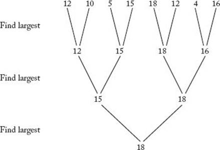
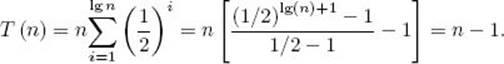
The second-to-last equality is obtained by applying the result in Example A.4 in Appendix A. This is the number of comparisons needed to complete the tournament. (Notice that we find the largest key with an optimal number of comparisons.) The largest key will have been involved in lg nmatches, which means that there will be lg n keys in its linked list. If we use Algorithm 8.2, it takes lg n − 1 comparisons to find the largest key in this linked list. That key is the second largest key. Therefore, the total number of comparisons needed to find the second largest key is
![]()
It is left as an exercise to show that, for n in general,
![]()
This performance is a substantial improvement over using Algorithm 8.2 twice to find the second-largest key. Recall that it takes 2n − 3 comparisons to do it that way. Can we obtain an algorithm that does even fewer comparisons? We use an adversary argument to show that we cannot.
![]() Theorem 8.9
Theorem 8.9
Any deterministic algorithm that can find the second largest of n keys in every possible input only by comparisons of keys must in the worst case do at least
![]()
Proof: To determine that a key is second largest, an algorithm must determine that it is the largest of the n − 1 keys besides the largest key. Let m be the number of comparisons won by the largest key. None of these comparisons is useful in determining that the second-largest key is the largest of the remaining n − 1 keys. Theorem 8.7 says that this determination requires at least n − 2 comparisons. Therefore, the total number of comparisons is at least m + n − 2. This means that, to prove the theorem, an adversary only needs to force the algorithm to make the largest key compete in at least ![]() lgn
lgn![]() comparisons. Our adversary’s strategy is to associate a node in a tree with each key. Initially, n single-node trees are created, one for each key. Our adversary uses the trees to give the result of the comparison of si and sj as follows:
comparisons. Our adversary’s strategy is to associate a node in a tree with each key. Initially, n single-node trees are created, one for each key. Our adversary uses the trees to give the result of the comparison of si and sj as follows:
• If both si and sj are roots of trees containing the same number of nodes, the answer is arbitrary. The trees are combined by making the key that is declared smaller a child of the other key.
• If both si and sj are roots of trees, and one tree contains more nodes than the other, the root of the smaller tree is declared smaller, and the trees are combined by making that root a child of the other root.
• If si is a root and sj is not, sj is declared smaller and the trees are not changed.
• If neither si nor sj is a root, the answer is consistent with previously assigned values and the trees are not changed.
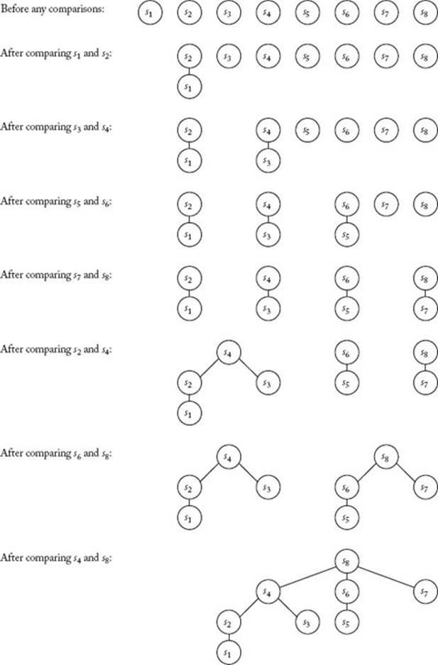
Figure 8.11 shows how trees would be combined when our adversary is presented with the Tournament method and an instance of size 8. When the choice is arbitrary, we make the key with the larger index the winner. Only the comparisons up to completion of the tournament are shown. After that, more comparisons would be done to find the largest of the keys that lost to the largest key, but the tree would be unchanged.
Let sizek be the number of nodes in the tree rooted at the largest key immediately after the kth comparison won by that key. Then
![]()
because the number of nodes in a defeated key’s tree can be no greater than the number of nodes in the victor’s tree. The initial condition is size0 = 1.
Figure 8.11 The trees created by our adversary in Theorem 8.9 when presented with the Tournament method and an input size of 8.
We can solve this recurrence using the techniques in Appendix B to conclude that
![]()
If a key is a root when the algorithm stops, it has never lost a comparison. Therefore, if two trees remain when the algorithm stops, two keys have never lost a comparison. At least one of those keys is not reported as the second-largest key. We can create a new input with all the other values the same, but with the values of the two roots changed so that the key that we know is not reported as the second largest is indeed the second-largest key. The algorithm would give the wrong answer for that input. So when the algorithm stops, all n keys must be in one tree. Clearly, the root of that tree must be the largest key. Therefore, if m is the total number of comparisons won by the largest key,
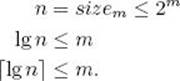
The last equality derives from the fact that m is an integer. This proves the theorem.
Because the Tournament method performs as well as our lower bound, it is optimal. We have again found a worthy adversary. No other adversary could produce a greater bound.
In the worst case, it takes at least n − 1 comparisons to find the largest key and at least n + ![]() lg n
lg n![]() − 2 comparisons to find the second-largest key. Any algorithm that finds the second-largest key must also find the largest key, because to know that a key is second largest, we must know that it has lost one comparison. That loss must be to the largest key. Therefore, it is not surprising that it is harder to find the second-largest key.
− 2 comparisons to find the second-largest key. Any algorithm that finds the second-largest key must also find the largest key, because to know that a key is second largest, we must know that it has lost one comparison. That loss must be to the largest key. Therefore, it is not surprising that it is harder to find the second-largest key.
• 8.5.4 Finding the kth-Smallest Key
In general, the Selection problem entails finding the kth-largest or kth-smallest key. So far, we’ve discussed finding the largest key, because it has seemed more appropriate for the terms used. That is, it seems appropriate to call the largest key a winner. Here we discuss finding the kth-smallest key because it makes our algorithms more lucid. For simplicity, we assume that the keys are distinct.
One way to find the kth-smallest key in Θ (n lg n) time is to sort the keys and return the kth key. We develop a method that requires fewer comparisons.
Recall that procedure partition in Algorithm 2.7, which is used in Quicksort (Algorithm 2.6), partitions an array so that all keys smaller than some pivot item come before it in the array and all keys larger than that pivot item come after it. The slot at which the pivot item is located is called thepivotpoint. We can solve the Selection problem by partitioning until the pivot item is at the kth slot. We do this by recursively partitioning the left subarray (the keys smaller than the pivot item) if k is less than pivotpoint, and by recursively partitioning the right subarray if k is greater than pivot-point. When k = pivotpoint, we’re done. This divide-and-conquer algorithm solves the problem by this method.
![]() Algorithm 8.5
Algorithm 8.5
Selection
Problem: Find the kth-smallest key in array S of n distinct keys.
Inputs: positive integers n and k where k ≤ n, array of distinct keys S indexed from 1 to n.
Outputs: the kth-smallest key in S. It is returned as the value of function selection.
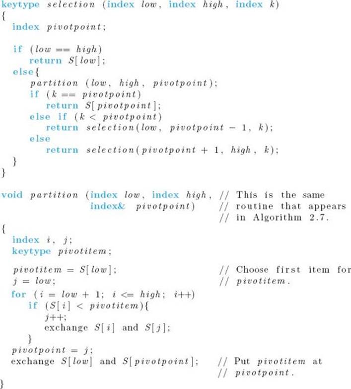
As with our recursive functions in previous chapters, n and S are not inputs to function selection. The top-level call to that function would be
![]()
As in Quicksort (Algorithm 2.6), the worst case occurs when the input to each recursive call contains one less item. This happens, for example, when the array is sorted in increasing order and k = n. Algorithm 8.5 therefore has the same worst-case time complexity as Algorithm 2.6, which means that the worst-case time complexity of the number of comparisons of keys done by Algorithm 8.5 is given by
![]()
Although the worst case is the same as that of Quicksort, we show next that Algorithm 8.5 performs much better on the average.
![]() Analysis of Algorithm 8.5
Analysis of Algorithm 8.5
![]() Average-Case Time Complexity (Selection)
Average-Case Time Complexity (Selection)
Basic operation: the comparison of S [i] with pivotitem in partition.
Input size: n, the number of items in the array.
We assume that all inputs are equally likely. This means that we assume that all values of k are entered with equal frequency and all values of pivotpoint are returned with equal frequency. Let p stand for pivotpoint. There are n outcomes for which there is no recursive call (that is, if p = k for k = 1, 2, … , n). There are two outcomes for which 1 is the input size in the first recursive call (that is, if p = 2 with k = 1, or p = n − 1 with k = n). There are 2(2) = 4 outcomes for which 2 is the input size in the first recursive call (that is, if p = 3 with k = 1 or 2, or p = n − 2 with k = n − 1 or n). Listed below are the numbers of outcomes for all the input sizes:
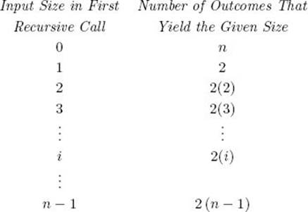
It is not hard to see that, for each of these input sizes, all allowable values of k appear with equal frequency. Recall from the every-case analysis of Algorithm 2.7 that the number of comparisons in procedure partition is n − 1. Therefore, the average is given by the following recurrence:
![]()
Using the result in Example A.1 in Appendix A and the fact that A (0) = 0, and simplifying, we have
![]()
Next we mimic the technique used in the average-case time complexity analysis of Algorithm 2.6 (Quicksort). That is, we multiply the expression for A (n) by n2, apply the expression to n − 1, subtract the expression for n − 1 from the one for n, and simplify to obtain
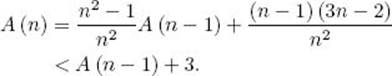
Because A (0) = 0, we have the following recurrence:
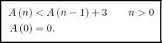
This recurrence can be solved using induction, as described in Section B.1 in Appendix B. The solution is
![]()
In the same way, we can use the recurrence to show that A (n) is bounded below by a linear function. Therefore,
![]()
It is straightforward to use the recurrence for A (n) to show that, for large values of n,
![]()
On the average, Algorithm 8.5 (Selection) does only a linear number of comparisons. Of course, the reason that this algorithm performs better on the average than Algorithm 2.6 (Quicksort) is that Quicksort has two calls to partition, whereas this algorithm has only one. However, they both degenerate into the same complexity when the input to the recursive call is n − 1. (In this case, Quicksort inputs an empty subarray on one side.) That time complexity is quadratic. If we could somehow prevent this from happening in Algorithm 8.5, we should be able to improve on worst-case quadratic time. Next we show how this is done.
The best thing would be if pivotpoint were to split the array in the middle, because then the input would be cut in half in each recursive call. Recall that the median of n distinct keys is the key such that half the keys are smaller and half are larger. (This is precise only if n is odd.) If we could always choose the median for pivotitem, we would have optimal performance. But how can we determine the median? In procedure partition, we could try calling function selection with an input consisting of the original array and k equal to about half the size of that array. And yet this will not help because we end up back in selection with an instance of the same size as our original instance. However, the following maneuver does work. Assume for the moment that n is an odd multiple of 5. (We need not use 5; this is discussed at the end of the section.) We divide the n keys into n/5 groups of keys, each containing five keys. We find the median of each of these groups directly. As you are asked to show in the exercises, this can be done with six comparisons. We then call function selection to determine the median of the n/5 medians. The median of the medians is not necessarily the median of the n keys, but, as Figure 8.12 shows, it is reasonably close. In that figure, the keys to the left of the smallest median (keys 2 and 3) must be less than the median of the medians, and the keys to the right of the largest median (keys 18 and 22) must be greater than the median of the medians. In general, the keys to the right of the smallest median (keys 8 and 12) and the keys to the left of the largest median (keys 6 and 14) could lie on either side of the median of medians. Notice that there are
Figure 8.12 Each bar represents a key. We do not know if the boldfaced keys are less than or greater than the median of the medians.
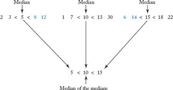
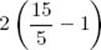
keys that could be on either side of the median of the medians. It is not hard to see that, whenever n is an odd multiple of 5, there are
keys that could lie on either side of the median of the medians. Therefore, there are at most
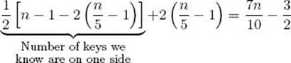
keys on one side of the median of the medians. We return to this result when we analyze the algorithm that uses this strategy. First we present the algorithm.
![]() Algorithm 8.6
Algorithm 8.6
Selection Using the Median
Problem: Find the kth-smallest key in the array S of n distinct keys.
Inputs: positive integers n and k where k ≤ n, array of distinct keys S indexed from 1 to n.
Outputs: the kth-smallest key in S. It is returned as the value of function select.
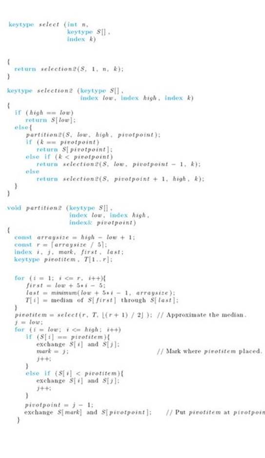
In Algorithm 8.6, unlike our other recursive algorithms, we show a simple function that calls our recursive function. The reason is that this simple function needs to be called in two places with different inputs. That is, it is called in procedure partition2 with T being the input, and globally as follows:
![]()
We also made the array an input to the recursive function selection2 because the function is called to process both the global array S and the local array T .
Next we analyze the algorithm.
![]() Analysis of Algorithm 8.6
Analysis of Algorithm 8.6
![]() Worst-Case Time CompIexity (Selection Using the Median)
Worst-Case Time CompIexity (Selection Using the Median)
Basic operation: the comparison of S [i] with pivotitem in partition2.
Input size: n, the number of items in the array.
For simplicity, we develop a recurrence assuming that n is an odd multiple of 5. The recurrence approximately holds for n in general. The components in the recurrence are as follows.
• The time in function selection2 when called from function selection2. As already discussed, if n is an odd multiple of 5, at most
![]()
end up on one side of pivotpoint, which means that this is the worst-case number of keys in the input to this call to selection2.
• The time in function selection2 when called from procedure partition2. The number of keys in the input to this call to selection2 is n/5.
• The number of comparisons required to find the medians. As mentioned previously, the median of five numbers can be found by making six comparisons. When n is a multiple of 5, the algorithm finds the median of exactly n/5 groups of five numbers. Therefore, the total number of comparisons required to find the medians is 6n/5.
• The number of comparisons required to partition the array. This number is n (assuming an efficient implementation of the comparison).
We have established the following recurrence:
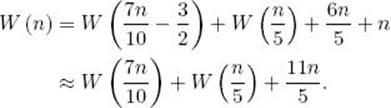
It is possible to show that the approximate equality holds even when n is not an odd multiple of 5. Of course, W (n) does not really have nonintegral inputs. However, considering such inputs simplifies our analysis. The recurrence does not suggest any obvious solution that can be used in an induction argument. Furthermore, it is not solvable by any of the other techniques in Appendix B. However, we can use a technique called constructive induction to obtain a candidate solution that can be used in an induction argument. That is, because we suspect that W (n) is linear, let’s assume that W (m) ≤ cm for all m < n and for some constant c. Then the recurrence implies that

Because we want to be able to conclude that W (n) ≤ cn, we need to solve
![]()
to determine a value of c that would work in an induction argument. The solution is
![]()
We then choose the smallest value of c that satisfies the inequality and proceed forward with a formal induction argument to show that when n is not small, the worst-case time complexity is approximately bound as follows:
![]()
Clearly, the inequality holds for n ≤ 5. It is left as an exercise to complete the induction argument. Theorem 8.7 says that linear time is required just to solve the case where k = 1. We can conclude that
![]()
We have successfully solved the Selection problem with an algorithm that is linear-time in the worst case. As mentioned previously, we did not have to divide the array into groups of size 5 to do this. If m is the group size, any odd value of m ≥ 5 yields a linear-time complexity. We now present the reason. Establishing the results we state is left for the exercises. For an arbitrary m, the recurrence for the worst-case time complexity is given by

where a is a positive constant. The sum of the coefficients of n in the expressions on the right is
![]()
It is straightforward that the expression on the right is less than 1 if and only if m > 3. It is possible to show that the recurrence
![]()
describes a linear equation if p + q < 1. Therefore, Recurrence 8.2 describes a linear equation for all m ≥ 5.
When m = 3, Recurrence 8.2 is as follows:
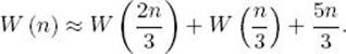
Using induction, it is possible to show that for this recurrence
![]()
Therefore, 5 is the smallest odd value of n that yields linear performance.
When m = 7, 9, or 11, the upper bound c on the time complexity is slightly smaller than when m = 5. The value of c increases very slowly as m increases beyond 11. For m not small, it is possible to show that c is approximated by 4 lg m. For example, if m = 100, the constant is about 4 lg 100 = 26.6.
Our linear-time algorithm for the Selection problem is from Blum, Floyd, Pratt, Rivest, and Tarjan (1973). The original version is more complex, but its number of comparisons of keys is only about 5.5n.
Hyafil (1976) has shown that a lower bound for finding the kth-smallest key in a set of n keys for k > 1 is given by
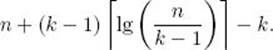
The proof can also be found in Horowitz and Sahni (1978). Notice that Theorem 8.9 is a special case of this result.
Other selection algorithms and lower bounds can be found in Schonhage, Paterson, and Pippenger (1976) and in Fussenegger and Gabow (1976).
• 8.5.5 A Probabilistic Algorithm for the Selection Problem
In obtaining lower bounds for algorithms, we have assumed the algorithms to be deterministic, but we mentioned that those bounds also hold for probabilistic algorithms. We close this discussion by presenting a probabilistic algorithm for the Selection problem to illustrate when such an algorithm is useful.
Section 5.3 presented a probabilistic algorithm—namely, a Monte Carlo algorithm for approximating the efficiency of a backtracking algorithm. Recall that a Monte Carlo algorithm does not necessarily give the correct answer. Rather, it provides an estimate of that answer, and the probability that the estimate is close to the correct answer increases as the time available to the algorithm increases. Here we show a different kind of probabilistic algorithm, called a Sherwood algorithm.
A Sherwood algorithm always gives the correct answer. Such an algorithm is useful when some deterministic algorithm runs much faster on the average than it does in the worst case. Recall that this is true of Algorithm 8.5 (Selection). The worst-case quadratic time is achieved in that algorithm when the pivotpoint for a particular input is repeatedly close to low or high in the recursive calls. This happens, for example, when the array is sorted in increasing order and k = n. Because this is not the case for most inputs, the algorithm’s average performance is linear. Suppose that, for a particular input, we choose the pivot item at random according to a uniform distribution. Then, when the algorithm is run for that input, the pivotpoint is more likely to be away from the endpoints than close to them. (Randonmess is reviewed in Section A.8 in Appendix A.) Therefore, linear performance is more likely. Because the number of comparisons is linear when averaged over all inputs, intuitively it seems that the expected value of the number of comparisons of keys done for a particular input should be linear when the pivot item is chosen at random according to a uniform distribution. We prove that this is the case, but first we stress the difference between this expected value and the average value obtained for Algorithm 8.5. Assuming that all possible inputs are presented in equal numbers, the average number of comparisons done by Algorithm 8.5 is linear. For any given input, Algorithm 8.5. always does the same number of comparisons, which is quadratic for some inputs. The Sherwood algorithm we are about to present does not do the same number of comparisons each time it executes on a given input. For any given input, it sometimes does a linear number of comparisons and sometimes does a quadratic number. However, if the algorithm is run many times using the same input, we can expect the average of the running times to be linear.
You may ask why we would want to use such an algorithm when Algorithm 8.6 (Selection Using the Median) guarantees linear performance. The reason is that Algorithm 8.6 has a high constant because of the overhead needed for approximating the median. For a given input, our Sherwoodalgorithm runs faster on the average than Algorithm 8.6. The decision about whether to use Algorithm 8.6 or the Sherwood algorithm depends on the needs of the particular application. If better average performance is most important, we should use the Sherwood algorithm. If, on the other hand, quadratic performance can never be tolerated, we should use Algorithm 8.6. We stress again the advantage of the Sherwood algorithm over Algorithm 8.5 (Selection). As long as the inputs are uniformly distributed, Algorithm 8.5 also performs better on the average than Algorithm 8.6. However, in some particular application, the inputs may always be ones that approach the worst case in Algorithm 8.5. In such an application, Algorithm 8.5 always exhibits quadratic-time performance. The Sherwood algorithm avoids this difficulty in any application by choosing the pivot item at random according to a uniform distribution.
Next we present the probabilistic (Sherwood) algorithm.
![]() Algorithm 8.7
Algorithm 8.7
ProbabiIistic Selection
Problem: Find the kth-smallest key in array S of n distinct keys.
Inputs: positive integers n and k where k ≤ n, array of distinct keys S indexed from 1 to n.
Outputs: the kth-smallest key in S. It is returned as the value of function selection3.
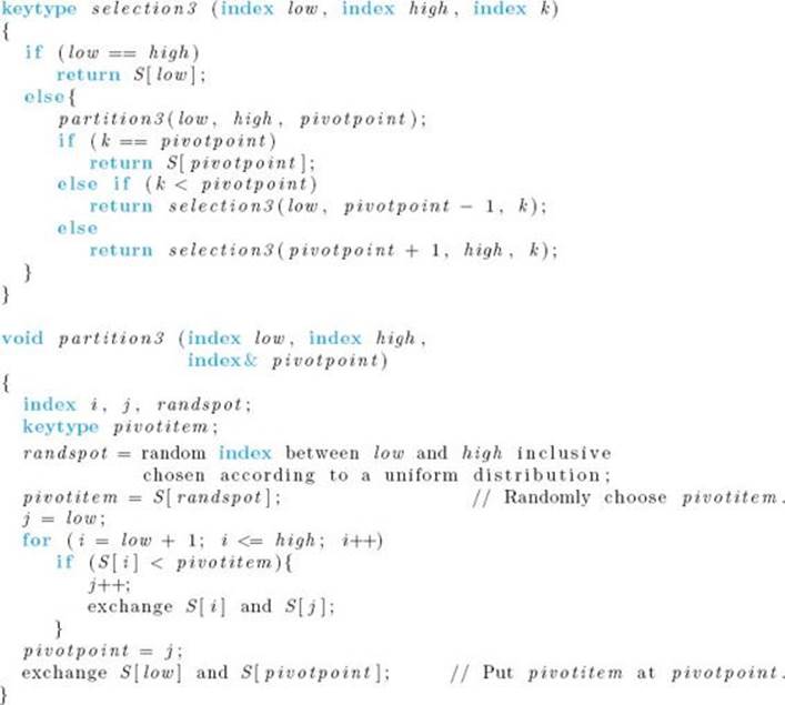
Algorithm 8.7 differs from Algorithm 8.5 only in its random choice of the pivot item. Next we prove that the expected value of the number of comparisons is linear for any input. This analysis must be different from the average-case analysis of Algorithm 8.5 (Selection), because in that analysis we assumed that all values of k are entered with equal frequency. We want to obtain a linear-time expected value for each input. Because each input has a specific value of k, we can’t assume that all values of k occur with equal frequency. We show that, independent of k, the expected value is linear.
![]() Analysis of Algorithm 8.7
Analysis of Algorithm 8.7
![]() Expected-Value Time Complexity (Probabilistic Selection)
Expected-Value Time Complexity (Probabilistic Selection)
Basic operation: the comparison of S [i] with pivotitem in partition.
Input size: n, the number of items in the array.
Given that we are looking for the kth-smallest key in an input of size n, the following table shows the size of the input and the new value of k in the first recursive call for each value of pivotpoint.
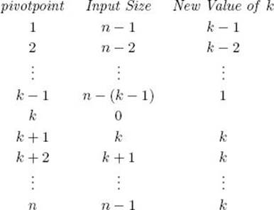
Because all values of pivotpoint are equally likely, we have the following recurrence for the expected value:
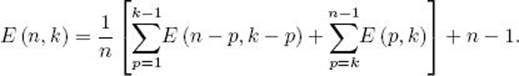
We can analyze this recurrence using constructive induction as we did in the worst-case analysis of Algorithm 8.6. That is, because we suspect that the recurrence is linear, we look for a value of c such that an induction argument should prove E (n, k) ≤ cn. This time, we show the induction argument, but we leave as an exercise the determination that c = 4 is the smallest constant that would work.
Induction base: Because no comparisons are done for n = 1,
![]()
Induction hypothesis: Suppose that, for all m < n and all k ≤ m,
![]()
Induction step: We need to show that, for all k ≤ n,
![]()
By the recurrence and the induction hypothesis,
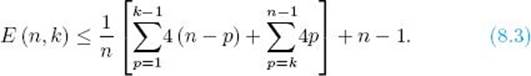
We have that
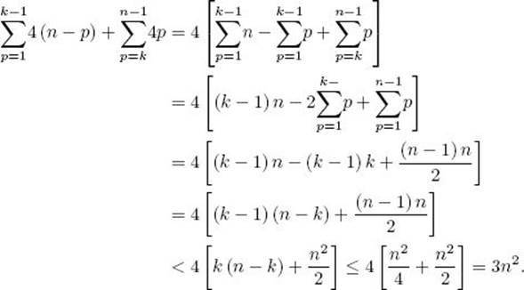
The third equality is obtained by twice applying the result of Example A.1 in Appendix A. The last inequality derives from the fact that, in general, k (n − k) ≤ n2/4. Plugging the result just obtained into Inequality 8.3, we have
![]()
We have shown that, independent of the value of k,
![]()
EXERCISES
Section 8.1
1. Let us assume that a search does not start at the beginning of a list when the Sequential Search algorithm (Algorithm 1.1) is used, but rather starts wherever the list index was left at the termination of the preceding search. Let us further assume that the item for which we are searching is selected randomly and independently of the destinations of previous searches. Under these assumptions, what would be the average number of comparisons?
2. Let S and T be two arrays of m and n elements, respectively. Write an algorithm that finds all the common elements and stores them in an array U. Show that this can be done in Θ (n + m) time.
3. Improve the Binary Search algorithm (Algorithm 1.5) assuming a successful search. Analyze your algorithm and show the results using order notation.
4. Show that, if x is in the array and is equally probable to be in each of the array slots, the average-case time complexity for Binary Search (Algorithm 1.5) is bounded approximately by
![]()
Hint: By Lemma 8.4, for some k, n − (2k − 1) is the number of nodes at the bottom level. The contribution to the TND for those nodes is equal to (n − 2k − 1) (k + 1). Add this expression to (k − 1) 2k + 1 (the formula established in the average-case analysis of Binary Search) to obtain the TNDfor the decision tree.
5. Suppose that all of the following 2n + 1 possibilities are equally probable:
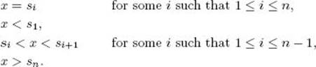
Show that the average-case time complexity of the Binary Search algorithm (Algorithm 1.5) is bounded approximately by
![]()
Hint: See the hint for Exercise 4.
6. Complete the proof of Lemma 8.6.
Section 8.2
7. Implement the Binary Search, Interpolation Search, and Robust Interpolation Search algorithms on your system and study their best-case, average-case, and worst-case performances using several problem instances.
8. Show that the average-case time complexity of Interpolation Search is in Θ(lg (lg n)), assuming the keys are uniformly distributed and that search key x is equally probable to be in each of the array slots.
9. Show that the worst-case time complexity of Interpolation Search is in Θ (lg n)2, assuming the keys are uniformly distributed and that search key x is equally probable to be in each of the array slots.
Section 8.3
10. Write an algorithm that finds the largest key in a binary search tree. Analyze your algorithm, and show the results using order notation.
11. Theorem 8.3 states that, for a successful search, the average search time over all inputs containing n keys, using binary search trees, is in Θ (lg n). Show that this result still holds if we consider an unsuccessful search as well.
12. Write an algorithm that deletes a node from a binary search tree considering all possible cases. Analyze your algorithm and show the results using order notation.
13. Write an algorithm that creates a 3–2 tree from a list of keys. Analyze your algorithm and show the results using order notation.
14. Write an algorithm that lists all the keys in a 3–2 tree in their natural order. Analyze your algorithm and show the results using order notation.
Section 8.4
15. Another clash (collision) resolution strategy is linear probing. In this strategy, all the elements are stored in the array of buckets (hash table). In the case of a clash, the table is searched for the next available (free) bucket. Show how linear probing resolves clashes that occur in the problem instance of Figure 8.8. (Linear probing is also known as closed hashing.)
16. Discuss the advantages and disadvantages of the two clash resolution strategies, open hashing and linear probing (see Exercise 15).
17. Write an algorithm to delete an element from a hash table that uses linear probing as its clash resolution strategy. Analyze your algorithm and show the results using order notation.
18. A rehashing scheme known as double hashing uses a second hash function in case of a clash. If the first hash function is h and the second hash function is s, the entire sequence of positions of the hash table that will be checked for an available bucket is given by the following equality, where piis the ith position in the sequence:
![]()
(% returns the remainder when the first operand is divided by the second.) Define a second hash function for the problem instance of Figure 8.8 and show the table after all the keys have been inserted into the hash table.
Section 8.5
19. Modify Algorithm 8.4 (Find Smallest and Largest Keys by Pairing Keys) so that it works when n (the number of keys in the given array) is odd and show that its time complexity is given by
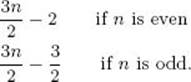
20. Complete the proof of Theorem 8.8. That is, show that a deterministic algorithm that finds the smallest and largest of n keys only by comparisons of keys must in the worst case do at least (3n − 3) /2 comparisons if n is odd.
21. Write an algorithm for the method discussed in Section 8.5.3 for finding the second-largest key in a given array.
22. Show that for n in general, the total number of comparisons needed by the method discussed in Section 8.5.3 for finding the second-largest key in a given array is
![]()
23. Show that the median of five numbers can be found by making six comparisons.
24. Use induction to show that the worst-case time complexity of Algorithm 8.6 (Selection Using the Median) is bounded approximately as follows:
![]()
25. Show that for an arbitrary m (group size), the recurrence for the worst-case time complexity of Algorithm 8.6 (Selection Using the Median) is given by
![]()
where a is a constant. This is Recurrence 8.2 in Section 8.5.4.
26. Use induction to show that W (n) ∈ Ω (n lg n) for the following recurrence. This is Recurrence 8.2 in Section 8.5.4 where m (group size) is 3.
![]()
27. Show that the constant c in the inequality
![]()
in the expected-value time complexity analysis of Algorithm 8.7 (Probabilistic Selection) cannot be less than 4.
28. Implement Algorithms 8.5, 8.6, and 8.7 (Selection algorithms for finding the kth-smallest key in an array) on your system and study their best-case, average-case, and worst-case performances using several problem instances.
29. Write a probabilistic algorithm that determines whether an array of n elements has a majority element (the element that appears the most). Analyze your algorithm and show the results using order notation.
Additional Exercises
30. Suppose a very large sorted list is stored in external storage. Assuming that this list cannot be brought into internal memory, develop a searching algorithm that looks for a key in this list. What major factor(s) should be considered when an external search algorithm is developed? Define the major factor(s), analyze your algorithm, and show the results using order notation.
31. Discuss the advantages of using each of the following instead of the other:
(a) A binary search tree with a balancing mechanism
(b) A 3–2 tree
32. Give at least two examples of situations in which hashing is not appropriate.
33. Let S and T be two arrays of n numbers that are already in nondecreasing order. Write an algorithm that finds the median of all 2n numbers whose time complexity is in Θ (lg n).
34. Write a probabilistic algorithm that factors any integer using the functions prime and factor. Function prime is a boolean function that returns “true” if a given integer is a prime number and returns “false” if it is not. Function factor is a function that returns a nontrivial factor of a given composite integer. Analyze your algorithm, and show the results using order notation.
35. List the advantages and disadvantages of all the searching algorithms discussed in this chapter.
36. For each of the searching algorithms discussed in this chapter, give at least two examples of situations in which the algorithm is the most appropriate.
All materials on the site are licensed Creative Commons Attribution-Sharealike 3.0 Unported CC BY-SA 3.0 & GNU Free Documentation License (GFDL)
If you are the copyright holder of any material contained on our site and intend to remove it, please contact our site administrator for approval.
© 2016-2026 All site design rights belong to S.Y.A.