Essential MATLAB for Engineers and Scientists (2013)

PART 2 Applications

CHAPTER 13 Simulation

Abstract

The objective of this chapter is to introduce you to simulation of real-life events. A simulation is a computer experiment which mirrors some aspect of the real world that appears to be based on random processes, or is too complicated to understand properly. (Whether events can be really random is actually a philosophical or theological question.) Some examples are: radio-active decay, rolling dice, bacteria division and traffic flow. The essence of a simulation program is that the programmer is unable to predict beforehand exactly what the outcome of the program will be, which is true to the event being simulated. For example, when you spin a coin, you do not know for sure what the result will be. Some of the examples just listed are examined in this chapter.

Keywords

Random processes; Random numbers; Simulation

CHAPTER OUTLINE

Random number generation

Seeding rand

Spinning coins

Rolling dice

Bacteria division

A random walk

Traffic flow

Normal (Gaussian) random numbers

Summary

Exercises

THE OBJECTIVE OF THIS CHAPTER IS TO INTRODUCE YOU TO:

■ Simulation of “real-life” events.

Simulation is an area of application where computers have come into their own. A simulation is a computer experiment which mirrors some aspect of the real world that appears to be based on random processes, or is too complicated to understand properly. (Whether events can be really random is actually a philosophical or theological question.) Some examples are: radio-active decay, rolling dice, bacteria division and traffic flow. The essence of a simulation program is that the programmer is unable to predict beforehand exactly what the outcome of the program will be, which is true to the event being simulated. For example, when you spin a coin, you do not know for sure what the result will be.

13.1. Random number generation

Random events are easily simulated in MATLAB with the function rand, which we have briefly encountered already. By default, rand returns a uniformly distributed pseudo-random number in the range . (A computer cannot generate truly random numbers, but they can be practically unpredictable.) rand can also generate row or column vectors, e.g., rand(1,5) returns a row vector of five random numbers (1 row, 5 column) as shown:

0.9501 0.2311 0.6068 0.4860 0.8913

If you generate more random numbers during the same MATLAB session, you will get a different sequence each time, as you would expect. However, each time you start a MATLAB session, the random number sequence begins at the same place (0.9501), and continues in the same way. This is not true to life, as every gambler knows. To produce a different sequence each time you start a session, rand can be initially seeded in a different way each time you start.

13.1.1. Seeding rand

The random number generator rand can be seeded with the statement

rand('state', n)

where n is any integer. (By default, n is set to 0 when a MATLAB session starts.) This is useful if you want to generate the same random sequence every time a script runs, e.g., in order to debug it properly. Note that this statement does not generate any random numbers; it only initializes the generator.

However, you can also arrange for n to be different each time you start MATLAB by using the system time. The function clock returns the date and time in a six-element vector with seconds to two decimal places, so the expression sum(100*clock) never has the same value (well, hardly ever). You can use it to seed rand as follows:

≫rand('state', sum(100*clock))

≫rand(1,7)

ans =

0.3637 0.2736 0.9910 0.3550 0.8501 0.0911 0.4493

≫rand('state', sum(100*clock))

≫rand(1,7)

ans =

0.9309 0.2064 0.7707 0.7644 0.2286 0.7722 0.5315

Theoretically rand can generate over 2¹⁴⁹² numbers before repeating itself.

13.2. Spinning coins

When a fair (unbiased) coin is spun, the probability of getting heads or tails is 0.5 (50%). Since a value returned by rand is equally likely to anywhere in the interval (0, 1) we can represent heads, say, with a value less than 0.5, and tails otherwise.

Suppose an experiment calls for a coin to be spun 50 times, and the results recorded. In real life you may need to repeat such an experiment a number of times; this is where computer simulation is handy. The following script simulates spinning a coin 50 times:

for i = 1:50

r = rand;

if r < 0.5

fprintf( 'H' )

else

fprintf( 'T' )

end

fprintf( '\n' ) % newline

Here is the output from two sample runs:

THHTTHHHHTTTTTHTHTTTHHTHTTTHHTTTTHTTHHTHHHHHHTTHTT

THTHHHTHTHHTTHTHTTTHHTTTTTTTHHHTTTHTHHTHHHHTTHTHTT

Note that it should be impossible in principle to tell from the output alone whether the experiment was simulated or real (if the random number generator is sufficiently random).

Can you see why it would be wrong to code the if part of the coin simulation like this:

if rand < 0.5 fprintf( 'H' ), end

if rand >= 0.5 fprintf( 'T' ), end

The basic principle is that rand should be called only once for each ‘event’ being simulated. Here the single event is spinning a coin, but rand is called twice. Also, since two different random numbers are generated, it is quite possible that both logical expressions will be true, in which case ‘H’ and ‘T’ will both be displayed for the same coin!

13.3. Rolling dice

When a fair dice is rolled, the number uppermost is equally likely to be any integer from 1 to 6. We saw in Counting random numbers (Chapter 5) how to use rand to simulate this. The following statement generates a vector with 10 random integers in the range 1–6:

d = floor( 6 * rand(1,10) + 1 )

Here are the results of two such simulations:

2 1 5 5 6 3 4 5 1 1

4 5 1 3 1 3 5 4 6 6

We can do statistics on our simulated experiment, just as if it were a real one. For example, we could estimate the mean of the number obtained when the dice is rolled 100 times, and the probability of getting a six, say.

13.4. Bacteria division

If a fair coin is spun, or a fair dice is rolled, the different events (e.g., getting ‘heads’, or a 6) happen with equal likelihood. Suppose, however, that a certain type of bacteria divides (into two) in a given time interval with a probability of 0.75 (75%), and that if it does not divide, it dies. Since a value generated by rand is equally likely to be anywhere between 0 and 1, the chances of it being less than 0.75 are precisely 75%. We can therefore simulate this situation as follows:

r = rand;

if r < 0.75

disp( 'I am now we' )

else

disp( 'I am no more' )

end

Again, the basic principle is that one random number should be generated for each event being simulated. The single event here is the bacterium's life history over the time interval.

13.5. A random walk

A seriously short-sighted sailor has lost his contact lenses returning from a symphony concert, and has to negotiate a jetty to get to his ship. The jetty is 50 paces long and 20 wide. He is in the middle of the jetty at the quay-end, pointing toward the ship. Suppose at every step he has a 60% chance of stumbling blindly toward the ship, but a 20% chance of lurching to the left or right (he manages to be always facing the ship). If he reaches the ship-end of the jetty, he is hauled aboard by waiting mates.

The problem is to simulate his progress along the jetty, and to estimate his chances of getting to the ship without falling into the sea. To do this correctly, we must simulate one random walk along the jetty, find out whether or not he reaches the ship, and then repeat this simulation 1000 times, say (if we have a fast enough computer!). The proportion of simulations that end with the sailor safely in the ship will be an estimate of his chances of making it to the ship. For a given walk we assume that if he has not either reached the ship or fallen into the sea after, say, 10000 steps, he dies of thirst on the jetty.

To represent the jetty, we set up co-ordinates so that the x-axis runs along the middle of the jetty with the origin at the quay-end. x and y are measured in steps. The sailor starts his walk at the origin each time. The structure plan and script are as follows:

1. Initialize variables, including number of walks n

2. Repeat n simulated walks down the jetty:

Start at the quay-end of the jetty

While still on the jetty and still alive repeat:

Get a random number R for the next step

If then

Move forward (to the ship)

Else if then

Move port (left)

Else

Move starboard

If he got to the ship then

Count that walk as a success

3. Compute and print estimated probability of reaching the ship

4. Stop.

% random walk

n = input( 'Number of walks: ' );

nsafe = 0; % number of times he makes it

for i = 1:n

steps = 0; % each new walk ...

x = 0; % ... starts at the origin

y = 0;

while x <= 50 & abs(y) <= 10 & steps < 1000

steps = steps + 1; % that's another step

r = rand; % random number for that step

if r < 0.6 % which way did he go?

x = x + 1; % maybe forward ...

elseif r < 0.8

y = y + 1; % ... or to port ...

else

y = y - 1; % ... or to starboard

end;

if x > 50

nsafe = nsafe + 1; % he actually made it this time!

end;

prob = 100 * nsafe / n;

disp( prob );

A sample run of 100 walks gave an 93% probability of reaching the ship.

You can speed up the script by about 20% if you generate a vector of 1 000 random numbers, say, at the start of each walk (with r = rand(1,1000);) and then reference elements of the vector in the while loop, e.g.,

if r(steps) < 0.6 ...

13.6. Traffic flow

A major application of simulation is in modeling the traffic flow in large cities, in order to test different traffic light patterns before inflicting them on the real traffic. In this example we look at a very small part of the problem: how to simulate the flow of a single line of traffic through one set of traffic lights. We make the following assumptions (you can make additional or different ones if like):

1. Traffic travels straight, without turning.

2. The probability of a car arriving at the lights in a particular second is independent of what happened during the previous second. This is called a Poisson process. This probability (call it p) may be estimated by watching cars at the intersection and monitoring their arrival pattern. In this simulation we take .

3. When the lights are green, assume the cars move through at a steady rate of, say, eight every ten seconds.

4. In the simulation, we will take the basic time period to be ten seconds, so we want a display showing the length of the queue of traffic (if any) at the lights every ten seconds.

5. We will set the lights red or green for variable multiples of ten seconds.

The situation is modeled with a script file traffic.m which calls three function files: go.m, stop.m, and prq.m. Because the function files need access to a number of base workspace variables created by traffic.m, these variables are declared global in traffic.m, and in all three function files.

In this example the lights are red for 40 s (red = 4) and green for 20 s (green = 2). The simulation runs for 240 s (n = 24).

The script, traffic.m, is as follows:

clc

clear % clear out any previous garbage!

global CARS GTIMER GREEN LIGHTS RED RTIMER T

CARS = 0; % number of cars in queue

GTIMER = 0; % timer for green lights

GREEN = 2; % period lights are green

LIGHTS = 'R'; % colour of lights

n = 48; % number of 10-sec periods

p = 0.3; % probability of a car arriving

RED = 4; % period lights are red

RTIMER = 0; % timer for red lights

for T = 1:n % for each 10-sec period

r = rand(1,10); % 10 seconds means 10 random numbers

CARS = CARS + sum(r < p); % cars arriving in 10 seconds

if LIGHTS == 'G'

go % handles green lights

else

stop % handles red lights

end;

The function files go.m, stop.m and prq.m (all separate M-files) are as follows:

% ----------------------------------------------------------

function go

global CARS GTIMER GREEN LIGHTS

GTIMER = GTIMER + 1; % advance green timer

CARS = CARS - 8; % let 8 cars through

if CARS < 0 % ... there may have been < 8

CARS = 0;

end;

prq; % display queue of cars

if GTIMER == GREEN % check if lights need to change

LIGHTS = 'R';

GTIMER = 0;

end;

% ----------------------------------------------------------

function stop

global LIGHTS RED RTIMER

RTIMER = RTIMER + 1; % advance red timer

prq; % display queue of cars

if RTIMER == RED % check if lights must be changed

LIGHTS = 'G';

RTIMER = 0;

end;

% ----------------------------------------------------------

function prq

global CARS LIGHTS T

fprintf( '%3.0f ', T ); % display period number

if LIGHTS == 'R' % display colour of lights

fprintf( 'R ' );

else

fprintf( 'G ' );

end;

for i = 1:CARS % display * for each car

fprintf( '*' );

end;

fprintf( '\n' ) % new line

Typical output looks like this:

1 R ****

2 R ********

3 R ***********

4 R **************

5 G **********

6 G *****

7 R ********

8 R *************

9 R ****************

10 R *******************

11 G **************

12 G **********

13 R **************

14 R *****************

15 R ********************

16 R ************************

17 G **********************

18 G ****************

19 R ******************

20 R **********************

21 R ************************

22 R ******************************

23 G **************************

24 G ***********************

From this particular run it seems that a traffic jam is building up, although more and longer runs are needed to see if this is really so. In that case, one can experiment with different periods for red and green lights in order to get an acceptable traffic pattern before setting the real lights to that cycle. Of course, we can get closer to reality by considering two-way traffic, and allowing cars to turn in both directions, and occasionally to break down, but this program gives the basic ideas.

13.7. Normal (Gaussian) random numbers

The function randn generates Gaussian or normal random numbers (as opposed to uniform) with a mean (μ) of 0 and a variance () of 1.

■ Generate 100 normal random numbers r with randn(1,100) and draw their histogram. Use the functions mean(r) and std(r) to find their mean and standard deviation (σ).

■ Repeat with 1000 random numbers. The mean and standard deviation should be closer to 0 and 1 this time.

The functions rand and randn have separate generators, each with its own seed.

Summary

■ A simulation is a computer program written to mimic a “real-life” situation which is apparently based on chance.

■ The pseudo-random number generator rand returns uniformly distributed random numbers in the range [0, 1), and is the basis of the simulations discussed in this chapter.

■ randn generates normally distributed (Gaussian) random numbers.

■ rand('state', n) enables the user to seed rand with any integer n. A seed may be obtained from clock, which returns the system clock time.

randn may be seeded (independently) in a similar way.

■ Each independent event being simulated requires one and only one random number.

Exercises

13.1 Write some statements to simulate spinning a coin 50 times using 0-1 vectors instead of a for loop. Hints: generate a vector of 50 random numbers, set up 0-1 vectors to represent the heads and tails, and use double and char to display them as a string of Hs and Ts.

13.2 In a game of Bingo the numbers 1 to 99 are drawn at random from a bag. Write a script to simulate the draw of the numbers (each number can be drawn only once), printing them ten to a line.

13.3 Generate some strings of 80 random alphabetic letters (lowercase only). For fun, see how many real words, if any, you can find in the strings.

13.4 A random number generator can be used to estimate π as follows (such a method is called a Monte Carlo method). Write a script which generates random points in a square with sides of length 2, say, and which counts what proportion of these points falls inside the circle of unit radius that fits exactly into the square. This proportion will be the ratio of the area of the circle to that of the square. Hence estimate π. (This is not a very efficient method, as you will see from the number of points required to get even a rough approximation.)

13.5 Write a script to simulate the progress of the short-sighted student in Chapter 6 (Markov Processes). Start him at a given intersection, and generate a random number to decide whether he moves toward the internet cafe or home, according to the probabilities in the transition matrix. For each simulated walk, record whether he ends up at home or in the cafe. Repeat a large number of times. The proportion of walks that end up in either place should approach the limiting probabilities computed using the Markov model described in Chapter 6. Hint: if the random number is less than 2/3 he moves toward the cafe (unless he is already at home or in the cafe, in which case that random walk ends), otherwise he moves toward home.

13.6 The aim of this exercise is to simulate bacteria growth.

Suppose that a certain type of bacteria divides or dies according to the following assumptions:

(a) during a fixed time interval, called a generation, a single bacterium divides into two identical replicas with probability p;

(b) if it does not divide during that interval, it dies;

(c) the offspring (called daughters) will divide or die during the next generation, independently of the past history (there may well be no offspring, in which case the colony becomes extinct).

Start with a single individual and write a script which simulates a number of generations. Take . The number of generations which you can simulate will depend on your computer system. Carry out a large number (e.g. 100) of such simulations. The probability of ultimate extinction, , may be estimated as the proportion of simulations that end in extinction. You can also estimate the mean size of the nth generation from a large number of simulations. Compare your estimate with the theoretical mean of .

Statistical theory shows that the expected value of the extinction probability is the smaller of 1, and . So for , is expected to be 1/3. But for , is expected to be 1, which means that extinction is certain (a rather unexpected result). You can use your script to test this theory by running it for different values of p, and estimating in each case.

13.7 Brian Hahn (the original author of this book) is indebted to a colleague, Gordon Kass, for suggesting this problem.

Dribblefire Jets Inc. make two types of aeroplane, the two-engined DFII, and the four-engined DFIV. The engines are terrible and fail with probability 0.5 on a standard flight (the engines fail independently of each other). The manufacturers claim that the planes can fly if at least half of their engines are working, i.e. the DFII will crash only if both its engines fail, while the DFIV will crash if all four, or if any three engines fail.

You have been commissioned by the Civil Aviation Board to ascertain which of the two models is less likely to crash. Since parachutes are expensive, the cheapest (and safest!) way to do this is to simulate a large number of flights of each model. For example, two calls of Math.random could represent one standard DFII flight: if both random numbers are less than 0.5, that flight crashes, otherwise it doesn't. Write a script which simulates a large number of flights of both models, and estimates the probability of a crash in each case. If you can run enough simulations, you may get a surprising result. (Incidentally, the probability of n engines failing on a given flight is given by the binomial distribution, but you do not need to use this fact in the simulation.)

13.8 Two players, A and B, play a game called Eights. They take it in turns to choose a number 1, 2 or 3, which may not be the same as the last number chosen (so if A starts with 2, B may only choose 1 or 3 at the next move). A starts, and may choose any of the three numbers for the first move. After each move, the number chosen is added to a common running total. If the total reaches 8 exactly, the player whose turn it was wins the game. If a player causes the total to go over 8, the other player wins. For example, suppose A starts with 1 (total 1), B chooses 2 (total 3), A chooses 1 (total 4) and B chooses 2 (total 6). A would like to play 2 now, to win, but he can't because B cunningly played it on the last move, so A chooses 1 (total 7). This is even smarter, because B is forced to play 2 or 3, making the total go over 8 and thereby losing.

Write a script to simulate each player's chances of winning, if they always play at random.

13.9 If r is a normal random number with mean 0 and variance 1 (as generated by randn), it can be transformed into a random number X with mean μ and standard deviation σ by the relation

In an experiment a Geiger counter is used to count the radio-active emissions of cobalt 60 over a 10-second period. After a large number of such readings are taken, the count rate is estimated to be normally distributed with a mean of 460 and a standard deviation of 20.

1. Simulate such an experiment 200 times by generating 200 random numbers with this mean and standard deviation. Plot the histogram (use 10 bins).

2. Repeat a few times to note how the histogram changes each time.

13.10 Radio-active carbon 11 has a decay-rate k of 0.0338 per min, i.e. a particular C¹¹ atom has a 3.38% chance of decaying in any one minute.

Suppose we start with 100 such atoms. We would like to simulate their fate over a period of 100 min, say. We want to end up with a bar graph showing how many atoms remain undecayed after 1, 2, …, 100 min.

We need to simulate when each of the 100 atoms decays. This can be done, for each atom, by generating a random number r for each of the 100 min, until either (that atom decays), or the 100 min is up. If the atom decayed at time , increment the frequency distribution by 1. will be the number of atoms decaying at time t minutes.

Now convert the number decaying each minute to the number remaining each minute. If there are n atoms to start with, after one minute, the number remaining will be , since is the number decaying during the first minute. The number remaining after two minutes will be . In general, the number remaining after t minutes will be (in MATLAB notation)

R(t) = n - sum( f(1:t) )

Write a script to compute and plot its bar graph. Superimpose on the bar graph the theoretical result, which is

Typical results are shown in Figure 13.1.

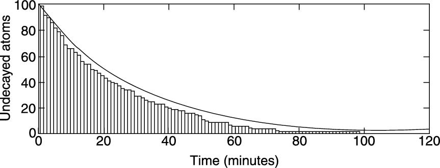
FIGURE 13.1 Radio-active decay of carbon 11: simulated and theoretical.