Essential MATLAB for Engineers and Scientists (2013)

PART 1

Essentials

CHAPTER 3

Program Design and Algorithm Development

Abstract

The objectives of this chapter are to introduce you to the art of program design. The top-down design process using a structure plan is elaborated to help you think about good problem-solving strategies as they relate to the design of procedures to effectively use MATLAB. Examples are provided, viz., the projectile problem and a harmonic oscillator problem. This chapter concludes with an introduction to user-defined MATLAB functions.

Keywords

Technical computing; Algorithm development; Program design

CHAPTER OUTLINE

The program design process

The projectile problem

Programming MATLAB functions

Inline objects: Harmonic oscillators

MATLAB function: y = f(x)

Summary

Exercise

THE OBJECTIVES OF THIS CHAPTER ARE TO INTRODUCE YOU TO:

■ Program design

■ User-defined MATLAB functions

This chapter is an introduction to the design of computer programs. The top-down design process is elaborated to help you think about good problem-solving strategies as they relate to the design of procedures for using software like MATLAB. We will consider the design of your own toolbox to be included among those already available with your version of MATLAB, such as Simulink, Symbolic Math, and Controls System. This is a big advantage of MATLAB (and tools like it); it allows you to customize your working environment to meet your own needs. It is not only the “mathematics handbook” of today's student, engineer, and scientist, it is also a useful environment to develop software tools that go beyond any handbook to help you to solve relatively complicated mathematical problems.

In the first part of this chapter we discuss the design process. In the second part we examine the structure plan—the detailed description of the algorithm to be implemented. We will consider relatively simple programs. However, the process described is intended to provide insight into what you will confront when you deal with more complex engineering, scientific, and mathematical problems during the later years of your formal education, your life-long learning, and your continuing professional education. In the third part we introduce the basic construct of a MATLAB function to help you develop more sophisticated programs.

To be sure, the examples examined so far have been logically simple. This is because we have been concentrating on the technical aspects of writing correct MATLAB statements. It is very important to learn how MATLAB does the arithmetic operations that form the basis of more complex programs. To design a successful program you need to understand a problem thoroughly and break it down into its most fundamental logical stages. In other words, you have to develop a systematic procedure or algorithm for solving it.

There are a number of methods that may assist in algorithm development. In this chapter we look at one, the structure plan. Its development is the primary part of the software (or code) design process because it is the steps in it that are translated into a language the computer can understand—for example, into MATLAB commands.

3.1. The program design process

Useful utilities translated into MATLAB (either sequences of command lines or functions, which are described later in the text) and saved as M-files in your working directory are your primary goals (see Figure 3.1). There are numerous toolboxes available through MathWorks (among others) on a variety of engineering and scientific topics. A great example is the Aerospace Toolbox, which provides reference standards, environmental models, and aerodynamic coefficients importing for advanced aerospace engineering designs. Explore the MathWorks Web site for products available (http://www.mathworks.com/).

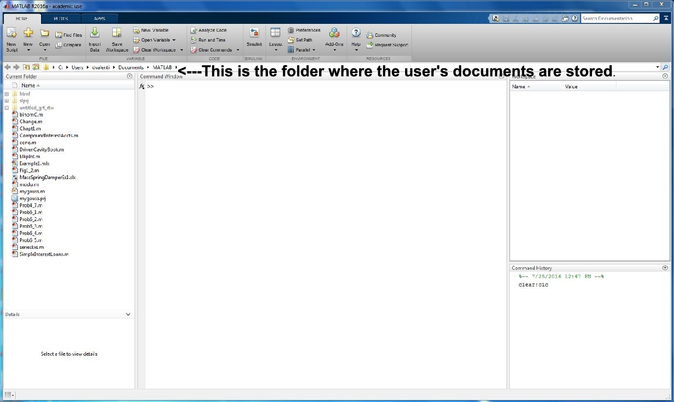
FIGURE 3.1 Creating your work folder: In your Users-Documents folder.

In your working directory, (e.g., the folder we are currently in, viz., \MATLAB), you will begin to accumulate a set of M-files that you have created as you use MATLAB.

Certainly, you want to be sure that the tools you save are reasonably well written (i.e., reasonably well designed). What does it mean to create well-written programs?

The goals in designing a software tool are that it works, it can easily be read and understood, and, hence, it can be systematically modified when required. For programs to work well they must satisfy the requirements associated with the problem or class of problems they are intended to solve. The specifications (i.e., the detailed description of purpose, or function, inputs, method of processing, outputs, and any other special requirements) must be known to design an effective algorithm or computer program, which must work completely and correctly. That is, all options should be usable without error within the limits of the specifications (see Figures 3.2 and 3.3).

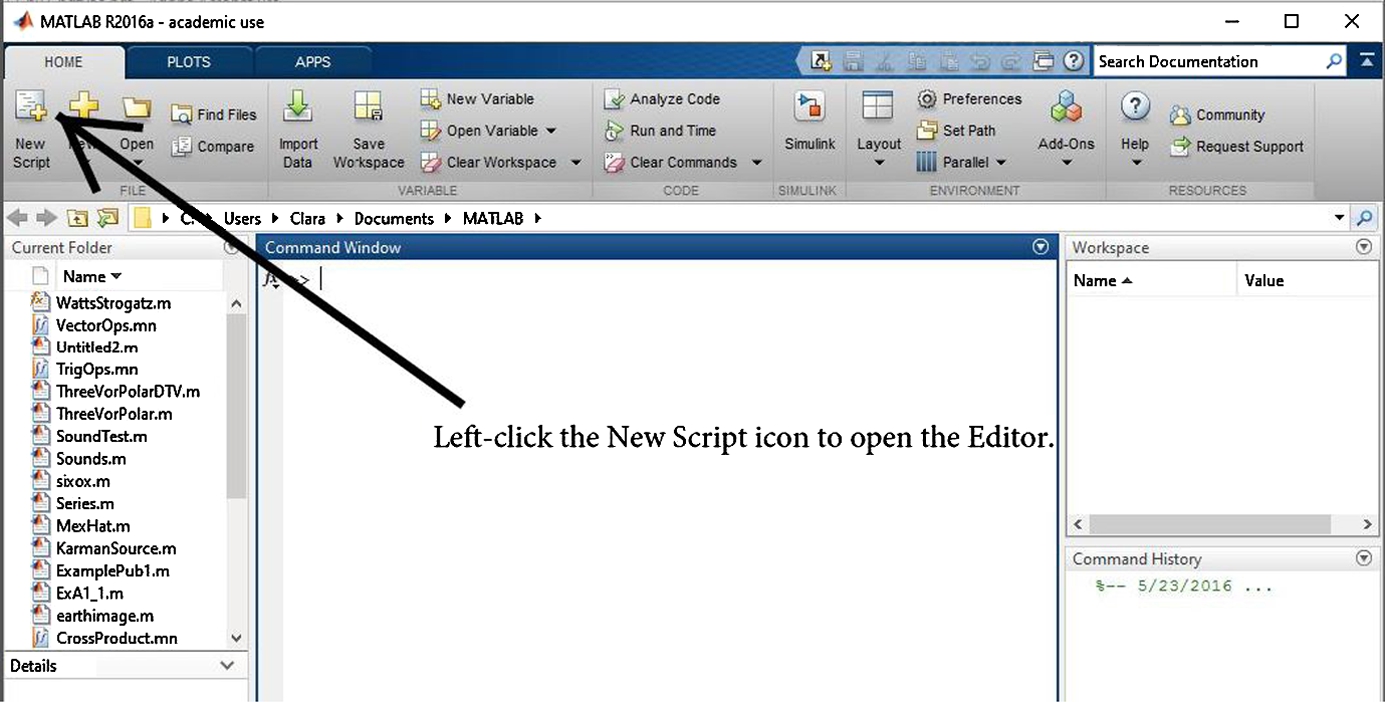
FIGURE 3.2 Creating your work folder.

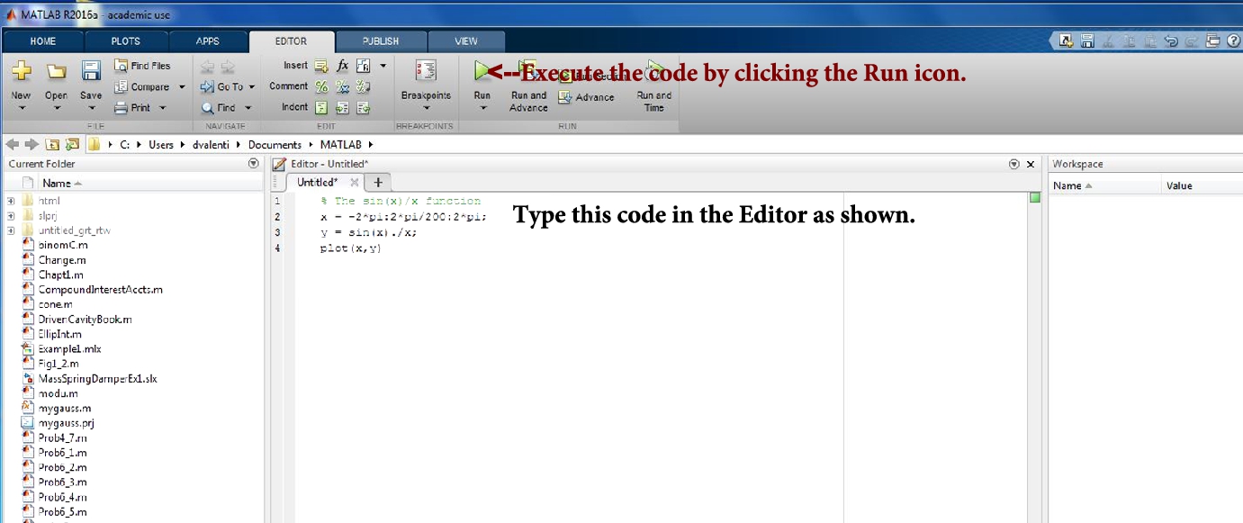
FIGURE 3.3 Creating your work folder: Entering, saving and executing a MATLAB M-file.

The program must be readable and hence clearly understandable. Thus, it is useful to decompose major tasks (or the main program) into subtasks (or subprograms) that do specific parts of it. It is much easier to read subprograms, which have fewer lines, than one large main program that doesn't segregate the subtasks effectively, particularly if the problem to be solved is relatively complicated. Each subtask should be designed so that it can be evaluated independently before it is implemented in the larger scheme of things (i.e., in the main program plan).

A well written code, when it works, is much more easily evaluated in the testing phase of the design process. If changes are necessary to correct sign mistakes and the like, they can be easily implemented. One thing to keep in mind when you add comments to describe the process programmed is this: Add enough comments and references so that a year from the time you write the program you know exactly what was done and for what purpose. Note that the first few comment lines in a script file are displayed in the Command Window when you type help followed by the name of your file (file naming is also an art).

The design process¹ is outlined next. The steps may be listed as follows:

Step 1 Problem analysis. The context of the proposed investigation must be established to provide the proper motivation for the design of a computer program. The designer must fully recognize the need and must develop an understanding of the nature of the problem to be solved.

Step 2 Problem statement. Develop a detailed statement of the mathematical problem to be solved with a computer program.

Step 3 Processing scheme. Define the inputs required and the outputs to be produced by the program.

Step 4 Algorithm. Design the step-by-step procedure in a top-down process that decomposes the overall problem into subordinate problems. The subtasks to solve the latter are refined by designing an itemized list of steps to be programmed. This list of tasks is the structure plan and is written in pseudo-code (i.e., a combination of English, mathematics, and anticipated MATLAB commands). The goal is a plan that is understandable and easily translated into a computer language.

Step 5 Program algorithm. Translate or convert the algorithm into a computer language (e.g., MATLAB) and debug the syntax errors until the tool executes successfully.

Step 6 Evaluation. Test all of the options and conduct a validation study of the program. For example, compare results with other programs that do similar tasks, compare with experimental data if appropriate, and compare with theoretical predictions based on theoretical methodology related to the problems to be solved. The objective is to determine that the subtasks and the overall program are correct and accurate. The additional debugging in this step is to find and correct logical errors (e.g., mistyping of expressions by putting a plus sign where a minus sign was supposed to be) and runtime errors that may occur after the program successfully executes (e.g., cases where division by zero unintentially occurs).

Step 7 Application. Solve the problems the program was designed to solve. If the program is well designed and useful, it can be saved in your working directory (i.e., in your user-developed toolbox) for future use.

3.1.1. The projectile problem

Step 1. Let us consider the projectile problem examined in first-semester physics. It is assumed that engineering and science students understand this problem (if it is not familiar to you, find a physics text that describes it or search the Web; the formulas that apply will be provided in step 2).

In this example we want to calculate the flight of a projectile (e.g., a golf ball) launched at a prescribed speed and a prescribed launch angle. We want to determine the trajectory of the flight path and the horizontal distance the projectile (or object) travels before it hits the ground. Let us assume zero air resistance and a constant gravitational force acting on the object in the opposite direction of the vertical distance from the ground. The launch angle, , is defined as the angle measured from the horizontal (ground plane) upward toward the vertical direction, , where implies a launch in the horizontal direction and implies a launch in the vertical direction (i.e., in the opposite direction of gravity). If is used as the acceleration of gravity, the launch speed, , must be entered in units of m/s. Thus, if the time, , is the time in seconds (s) from the launch time of , the distance traveled in x (the horizontal direction) and y (the vertical direction) is in meters (m).

We want to determine the time it takes the projectile, from the start of motion, to hit the ground, the horizontal distance traveled, and the shape of the trajectory. In addition, we want to plot the speed of the projectile versus the angular direction of this vector. We need, of course, the theory (or mathematical expressions) that describes the solution to the zero-resistance projectile problem in order to develop an algorithm to obtain solutions to it.

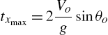
Step 2. The mathematical formulas that describe the solution to the projectile problem are provided in this step. Given the launch angle and launch speed, the horizontal distance traveled from , which is the coordinate location of the launcher, is

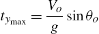
The time from at launch for the projectile to reach (i.e., its range) is

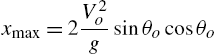
The object reaches its maximum altitude,

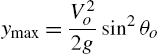
at time

The horizontal distance traveled when the object reaches the maximum altitude is .

The trajectory (or flight path) is described by the following pair of coordinates at a given instant of time between and :

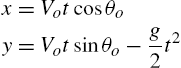
We need to solve these equations over the range of time for prescribed launch conditions and . Then the maximum values of the altitude and the range are computed along with their respective arrival times. Finally, we want to plot V versus θ, where

and

We must keep in mind when we study the solutions based on these formulas that the air resistance was assumed negligible and the gravitational acceleration was assumed constant.

Step 3. The required inputs are g, , , and a finite number of time steps between and the time the object returns to the ground. The outputs are the range and time of flight, the maximum altitude and the time it is reached, and the shape of the trajectory in graphical form.

Steps 4 and 5. The algorithm and structure plan developed to solve this problem are given next as a MATLAB program, because it is relatively straightforward and the translation to MATLAB is well commented with details of the approach applied to its solution (i.e., the steps of the structure plan are enumerated). This plan, and M-file, of course, is the summary of the results developed by trying a number of approaches during the design process, and thus discarding numerous sheets of scratch paper before summarizing the results! (There are more explicit examples of structure plans for your review and investigation in the next section of this chapter.) Keep in mind that it was not difficult to enumerate a list of steps associated with the general design process, that is, the technical problem solving. However, it is certainly not so easy to implement the steps because they draw heavily on your technical-solution design experience. Hence, we must begin by studying the design of relatively simple programs like the one described in this section.

The evaluated and tested code is as follows:

% The proctile problem with zero air resistance

% in a gravitational field with constant g.

% Written by Daniel T. Valentine .. September 2006

% Revised by D. T. Valentine ........... 2012/2016

% An eight-step structure plan applied in MATLAB:

%

% 1. Define the input variables.

%

g = 9.81; % Gravity in m/s/s.

vo = input('What is the launch speed in m/s? ')

tho = input('What is the launch angle in degrees? ')

tho = pi*tho/180; % Conversion of degrees to radians.

%

% 2. Calculate the range and duration of the flight.

%

txmax = (2*vo/g) * sin(tho);

xmax = txmax * vo * cos(tho);

%

% 3. Calculate the sequence of time steps to compute

% trajectory.

%

dt = txmax/100;

t = 0:dt:txmax;

%

% 4. Compute the trajectory.

%

x = (vo * cos(tho)) .* t;

y = (vo * sin(tho)) .* t - (g/2) .* t.^2;

%

% 5. Compute the speed and angular direction of the

% projectile. Note that vx = dx/dt, vy = dy/dt.

%

vx = vo * cos(tho);

vy = vo * sin(tho) - g .* t;

v = sqrt(vx.*vx + vy.*vy); % Speed

th = (180/pi) .* atan2(vy,vx); % Angular direction

%

% 6. Compute the time and horizontal distance at the

% maximum altitude.

%

tymax = (vo/g) * sin(tho);

xymax = xmax/2;

ymax = (vo/2) * tymax * sin(tho);

%

% 7. Display in the Command Window and on figures the ouput.

%

disp(['Range in meters = ',num2str(xmax),',' ...

' Duration in seconds = ', num2str(txmax)])

disp(' ')

disp(['Maximum altitude in meters = ',num2str(ymax), ...

', Arrival at this altitude in seconds = ', num2str(tymax)])

plot(x,y,'k',xmax,y(size(t)),'o',xmax/2,ymax,'o')

title(['Projectile flight path: v_o = ', num2str(vo),' m/s' ...

', \theta_o = ', num2str(180*tho/pi),' degrees'])

xlabel('x'), ylabel('y') % Plot of Figure 3.4.

figure % Creates a new figure.

plot(v,th,'r')

title('Projectile speed vs. angle')

xlabel('V'), ylabel('\theta') % Plot of Figure 3.5.

%

% 8. Stop.

Steps 6 and 7. The program was evaluated by executing a number of values of the launch angle and launch speed within the required specifications. The angle of 45 degrees was checked to determine that the maximum range occurred at this angle for all specified launch speeds. This is well known for the zero air resistance case in a constant g force field. Executing this code for m/s and degrees, the trajectory and the plot of orientation versus speed in Figures 3.4 and 3.5, respectively, were produced.

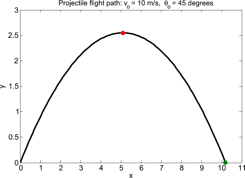
FIGURE 3.4 Projectile trajectory.

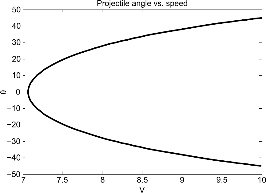
FIGURE 3.5 Projectile angle versus speed.

How can you find additional examples of MATLAB programs (good ones or otherwise) to help develop tools to solve your own problems? We all recognize that examples aren't a bad way of learning to use tools. New tools are continually being developed by the users of MATLAB. If one proves to be of more general use, MathWorks may include it in their list of products (if, of course, the tools' author desires this). There are also many examples of useful scripts that are placed on the Web for anyone interested in them. They, of course, must be evaluated carefully since it is the user's responsibility, not the creator's, to ensure the correctness of their results. This responsibility holds for all tools applied by the engineer and the scientist. Hence, it is very important (just as in using a laboratory apparatus) that users prove to themselves that the tool they are using is indeed valid for the problem they are trying to solve.

To illustrate how easy it is to find examples of scripts, the author typed MATLAB examples in one of the available search engines and found the following (among many others):

t = 0:.1:2*pi;

subplot(2,2,1)

plot(t,sin(t))

subplot(2,2,2)

plot(t,cos(t))

subplot(2,2,3)

plot(t,exp(t))

subplot(2,2,4)

plot(t,1./(1+t.^2))

This script illustrates how to put four plots in a single figure window. To check that it works, type each line in the Command Window followed by Enter. Note the position of each graphic; location is determined by the three integers in the subplot function list of arguments. Search Help via the question mark (?) for more information on subplot.

3.2. Programming MATLAB functions

MATLAB enables you to create your own function M-files. A function M-file is similar to a script file in that it also has a .m extension. However, a function M-file differs from a script file in that a function M-file communicates with the MATLAB workspace only through specially designated input and output arguments. Functions are indispensable tools when it comes to breaking a problem down into manageable logical pieces.

Short mathematical functions may be written as one-line inline objects. This capability is illustrated by example in the next subsection. In the subsequent subsection essential ideas embodied in the creation of a MATLAB function M-file will be introduced. (Further details on writing functions are provided in Chapter 4.)

3.2.1. Inline objects: Harmonic oscillators

If two coupled harmonic oscillators, e.g., two masses connected with a spring on a very smooth table, are considered as a single system, the output of the system as a function of time t could be given by something like

(3.1)

You can represent at the command line by creating an inline object as follows:

h = inline( 'cos(8*t) + cos(9*t)' );

Now write some MATLAB statements in the Command Window which use your function h to draw the graph in Figure 3.6 e.g.,

x = 0 : 20/300 : 20;

plot(x, h(x)), grid

Note:

■ The variable t in the inline definition of h is the input argument. It is essentially a ‘dummy’ variable, and serves only to provide input to the function from the outside world. You can use any variable name here; it doesn't have to be the same as the one used when you invoke (use) the function.

■ You can create functions of more than one argument with inline. For example,

f1 = inline( 'x.^2 + y.^2', 'x', 'y' );

f1(1, 2)

ans =

5

Note that the input values of x and y can be arrays and, hence, the output f1 will be an array of the same size as x and y. For example, after executing the previous two command lines to get the ans = 5, try the following:

x = [1 2 3; 1 2 3]; y = [4 5 6; 4 5 6];

f1(x,y)

ans =

17 29 45

17 29 45

The answer is an element-by-element operation that leads to the value of the function for each combination of like-located array elements.

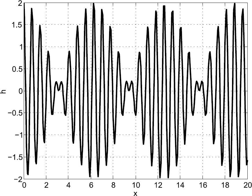
FIGURE 3.6 cos(8t) +cos(9t).

3.2.2. MATLAB function: y = f(x)

The essential features of a MATLAB function are embodied in the following example. Let us consider the function y defined by the relationship , i.e., y is a function of x. The construction of a function file starts with the declaration of a function command. This is followed by the formula that is the function of interest that you wish to substitute a particular value of x to get the corresponding value of y. The structure plan for the evaluation of a particular algebraic function is as follows:

1. function y = f(x) % where $x$ is the input and $y$ is the output.

2. y = x.^3 - 0.95*x;

3. end % This is not necessary to include; however, it plays the role of STOP.

The function M-file created based on this plan is as follows:

function y = f(x)

% where $x$ is the input and $y$ is the output.|

y = x.^3 - 0.95*x;

end % This is not necessary to include; however, it plays the

role of STOP.

It was saved as f.m. After saving it, it was used as follows in the Command Window. Try the following example:

>> f(2)

ans =

6.1000

Let us next create a function that takes as input the three coefficients of the quadratic equation, viz.,

We want the determine the two roots of this equation, i.e., we want to determine the solution to this equation. One way of dealing with this problem is to apply the known solutions of the quadratic equation. Let us do this by creating a function file by following the structure plan for the complete algorithm for finding the solution(s) x, given the coefficients a, b and c given as follows:

QUADRATIC EQUATION STRUCTURE PLAN

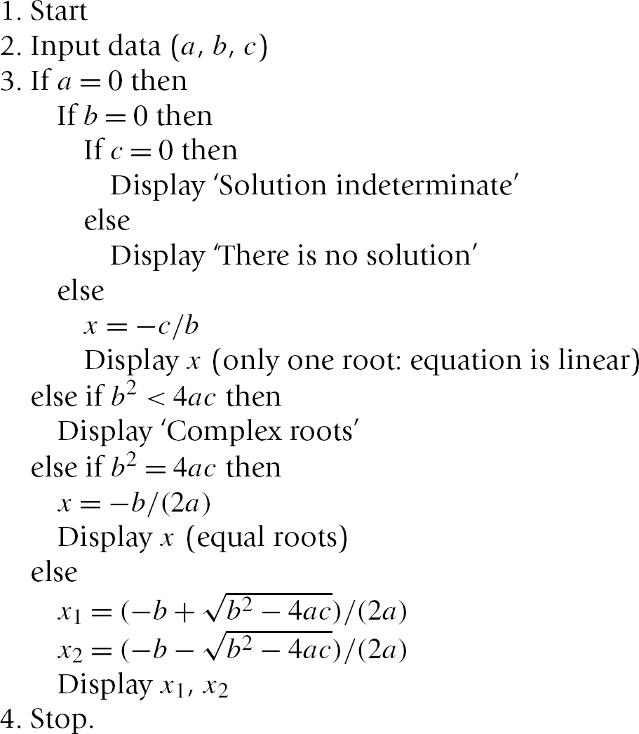
A function file based on this plan is as follows:

function x = quadratic(a,b,c)

% Equation:

% a*x^2 + b*x + c = 0

% Input: a,b,c

% Output: x = [x1 x2], the two solutions of

% this eequation.

if a==0 & b==0 & c==0

disp(' ')

disp('Solution indeterminate')

elseif a==0 & b==0

disp(' ')

disp('There is no solution')

elseif a==0

disp(' ')

disp('Only one root: equation is linear')

disp(' x ')

x1 = -c/b;

x2 = NaN;

elseif b^2 < 4*a*c

disp(' ')

disp(' x1, x2 are complex roots ')

disp(' x1 x2')

x1 = (-b + sqrt(b^2 - 4*a*c))/(2*a);

x2 = (-b - sqrt(b^2 - 4*a*c))/(2*a);

elseif b^2 == 4*a*c

x1 = -b/(2*a);

x2 = x1;

disp('equal roots')

disp(' x1 x2')

else

x1 = (-b + sqrt(b^2 - 4*a*c))/(2*a);

x2 = (-b - sqrt(b^2 - 4*a*c))/(2*a);

disp(' x1 x2')

end

if a==0 & b==0 & c==0

elseif a==0 & b==0

else

disp([x1 x2]);

end

end

This function is saved with the file name quadratic.m.

>> a = 4; b = 2; c = -2;

>> quadratic(a,b,c)

x1 x2

0.5000 -1.0000

>> who

Your variables are:

a b c

The two roots in this case are real. It is a useful exercise to test all possibilities to evaluate whether or not this function successfully deals with all quadratic equations with constant coefficients. The purpose of this example was to illustrate how to construct a function file. Note that the only variables in the Workspace are the coefficients a b c. The variables defined and needed in the function are not included in the Workspace. Hence, functions do not clutter the Workspace with the variables only needed in the function itself to execute the commands within it.

Summary

■ An algorithm is a systematic logical procedure for solving a problem.

■ A structure plan is a representation of an algorithm in pseudo-code.

■ A function M-file is a script file designed to handle a particular task that may be activated (invoked) whenever needed.

Exercise

The problems in these exercises should all be structure-planned before being written up as MATLAB programs (where appropriate).

3.1 The structure plan in this example defines a geometric construction. Carry out the plan by sketching the construction:

1. Draw two perpendicular x- and y-axes

2. Draw the points A (10, 0) and B (0, 1)

3. While A does not coincide with the origin repeat: Draw a straight line joining A and B Move A one unit to the left along the x-axis Move B one unit up on the y-axis

4. Stop

3.2 Consider the following structure plan, where M and N represent MATLAB variables:

1. Set M = 44 and N = 28

2. While M not equal to N repeat: While repeat: Replace value of M by  While repeat: Replace value of N by

3. Display M

4. Stop

(a) Work through the structure plan, sketching the contents of M and N during execution. Give the output.

(b) Repeat (a) for and .

(c) What general arithmetic procedure does the algorithm carry out (try more values of M and N if necessary)?

3.3 Write a program to convert a Fahrenheit temperature to Celsius. Test it on the data in Exercise 2.11 (where the reverse conversion is done).

3.4 Write a script that inputs any two numbers (which may be equal) and displays the larger one with a suitable message or, if they are equal, displays a message to that effect.

3.5 Write a script for the general solution to the quadratic equation . Use the structure plan in Section 3.2.2. Your script should be able to handle all possible values of the data a, b, and c. Try it out on the following values:

(a) 1, 1, 1 (complex roots)

(b) 2, 4, 2 (equal roots of −1.0)

(c) 2, 2, −12 (roots of 2.0 and −3.0)

The structure plan in Section 3.2.2 is for programming languages that cannot handle complex numbers. MATLAB can. Adjust your script so that it can also find complex roots. Test it on case (a); the roots are .

3.6 Develop a structure plan for the solution to two simultaneous linear equations (i.e., the equations of two straight lines). Your algorithm must be able to handle all possible situations; that is, lines intersecting, parallel, or coincident. Write a program to implement your algorithm, and test it on some equations for which you know the solutions, such as

(, ).

Hint: Begin by deriving an algebraic formula for the solution to the system:

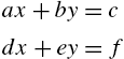
The program should input the coefficients a, b, c, d, e, and f.

We will see in Chapter 6 that MATLAB has a very elegant way of solving systems of equations directly, using matrix algebra. However, it is good for the development of your programming skills to do it the long way, as in this exercise.

3.7 We wish to examine the motion of a damped harmonic oscillator. The small amplitude oscillation of a unit mass attached to a spring is given by the formula , where is the square of the natural frequency of the oscillation with damping (i.e., with resistance to motion); is the square of the natural frequency of undamped oscillation; k is the spring constant; and R is the damping coefficient. Consider and vary R from 0 to 2 in increments of 0.5. Plot y versus t for t from 0 to 10 in increments of 0.1.

Hint: Develop a solution procedure by working backwards through the problem statement. Starting at the end of the problem statement, the solution procedure requires the programmer to assign the input variables first followed by the execution of the formula for the amplitude and ending with the output in graphical form.

3.8 Let's examine the shape of a uniform cable hanging under its own weight. The shape is described by the formula . This shape is called a uniform catenary. The parameter c is the vertical distance from where the bottom of the catenary is located. Plot the shape of the catenary between and for . Compare this with the same result for .

Hint: The hyperbolic cosine, cosh, is a built-in MATLAB function that is used in a similar way to the sine function, sin.